SKD006 - Coefficient interpretation

SKD006 is a tip about interpretation. This check flags that on mixed-scale features, raw coefficient magnitudes are not directly comparable across columns, and after standardization they are comparable but no longer expressed in the original feature units. Which path you take depends on what you want to read from the coefficients. See also scikit-learn’s example on linear model coefficient interpretation.

When reading coefficients under SKD006, think of:

• standardizing the inputs when you want coefficients that are comparable across features (see scale matters),

• multiplying each coefficient by the feature’s standard deviation for an “effect per one std” without refitting,

• relying on a scale-invariant ranking such as permutation importance when you need importance that does not depend on coefficient units.

We use California housing regression with Ridge on raw numeric columns. The goal is to interpret effect sizes without mistaking scale differences for importance.

Load the California housing dataset

Median income is measured in 10k USD blocks, latitude in degrees, and population in head counts. Fitting Ridge on these raw columns produces coefficients whose magnitudes reflect units as much as predictive strength.

from skrub.datasets import fetch_california_housing

housing = fetch_california_housing()
X, y = housing.X, housing.y

TableReport highlights the range differences across columns.

from skrub import TableReport

TableReport(X)

Please enable javascript

The skrub table reports need javascript to display correctly. If you are displaying a report in a Jupyter notebook and you see this message, you may need to re-execute the cell or to trust the notebook (button on the top right or "File > Trust notebook").

TableReport(y)

Please enable javascript

The skrub table reports need javascript to display correctly. If you are displaying a report in a Jupyter notebook and you see this message, you may need to re-execute the cell or to trust the notebook (button on the top right or "File > Trust notebook").

A single TrainTestSplit with a 20 % test set feeds every evaluation below.

from skore import TrainTestSplit

splitter = TrainTestSplit(test_size=0.2, random_state=42)

Trigger SKD006 with Ridge on raw mixed-scale features

Ridge with a moderate alpha fits quickly on unscaled inputs. SKD006 indicates that the features are not on the same scale, so raw coefficient magnitudes should not be read as a ranking of importance.

from sklearn.linear_model import Ridge
from skore import evaluate

report = evaluate(
    Ridge(alpha=1.0),
    X=X,
    y=y,
    splitter=splitter,
)
report

Ridge()

In a Jupyter environment, please rerun this cell to show the HTML representation or trust the notebook.
On GitHub, the HTML representation is unable to render, please try loading this page with nbviewer.org.

Please enable javascript

The skrub table reports need javascript to display correctly. If you are displaying a report in a Jupyter notebook and you see this message, you may need to re-execute the cell or to trust the notebook (button on the top right or "File > Trust notebook").

Find SKD006 in the Tips tab below.

report.checks.summarize()

Let us inspect coefficients with coefficients(), and compare each coefficient’s magnitude to the feature’s typical range (or standard deviation): a large coefficient on a small-scale column is not necessarily more important than a small coefficient on a large-scale column such as Population.

Unscaled coefficients are still useful on their own: they answer “if I change this feature by one unit in its original scale, how much does the prediction change in target units?” They are misleading regarding feature importance.

coef_display = report.inspection.coefficients()
coef_display.frame()

	feature	coefficient
0	Intercept	-37.019420
1	MedInc	0.448511
2	HouseAge	0.009726
3	AveRooms	-0.123014
4	AveBedrms	0.781417
5	Population	-0.000002
6	AveOccup	-0.003526
7	Latitude	-0.419787
8	Longitude	-0.433681

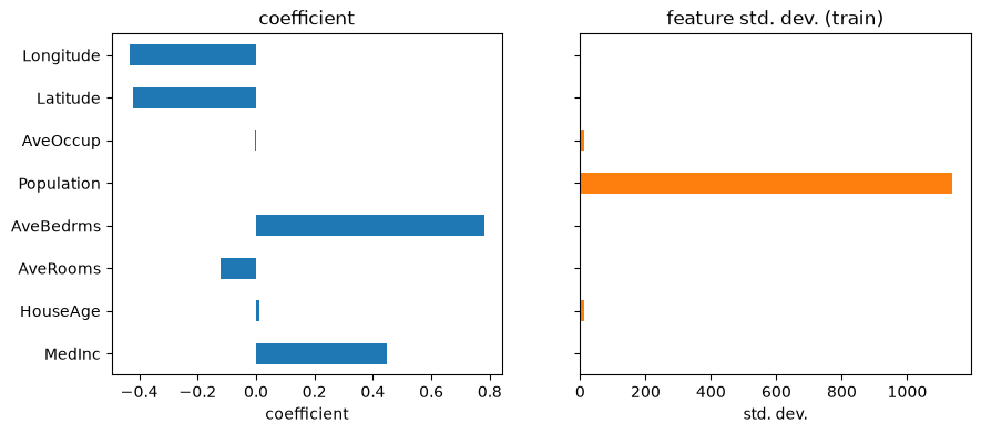
Side by side, the raw coefficient magnitudes and the feature standard deviations tell different stories. For instance, Population has a tiny coefficient because a one-person change is negligible on a head-count scale, even though the column varies a lot across districts.

import pandas as pd

coef = coef_display.frame(include_intercept=False).set_index("feature")
feature_std = report.X_train.std().rename("feature std. dev. (train)")

df = pd.concat([coef, feature_std], axis=1)
axes = df.plot.barh(
    subplots=True,
    layout=(1, 2),
    legend=False,
    sharey=True,
    sharex=False,
    figsize=(10, 4),
)
axes[0, 0].set_xlabel("coefficient")
_ = axes[0, 1].set_xlabel("std. dev.")

Scale coefficients by feature standard deviation

Recall the pitfall above: when the model was trained on features with different dynamic ranges, you cannot compare features by looking at raw coefficients alone. Multiplying each fitted coefficient by its feature standard deviation gives an “effect per one standard deviation” that is comparable across columns without refitting. See scikit-learn’s discussion of scale matters.

comparable = coef.copy()
comparable["effect per std. dev."] = comparable["coefficient"] * feature_std
_ = comparable.plot.barh()

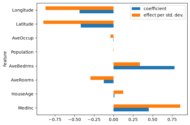
That rescaling erases the surprises from the side-by-side bars above. The large raw AveBedrms coefficient shrinks once multiplied by its small standard deviation, so it drops in the ranking while other features become, in comparison, more important.

Standardize inputs in a pipeline

StandardScaler inside a Pipeline puts every feature on a common scale at fit time, so coefficients become directly comparable as “effect per one standard deviation.” That is useful for ranking features, but you lose statements in original units (for example, “one extra year of age”).

from sklearn.pipeline import Pipeline
from sklearn.preprocessing import StandardScaler

report_scaled = evaluate(
    Pipeline([("scale", StandardScaler()), ("ridge", Ridge(alpha=1.0))]),
    X=X,
    y=y,
    splitter=splitter,
)
report_scaled

Pipeline(steps=[('scale', StandardScaler()), ('ridge', Ridge())])

In a Jupyter environment, please rerun this cell to show the HTML representation or trust the notebook.
On GitHub, the HTML representation is unable to render, please try loading this page with nbviewer.org.

Please enable javascript

The skrub table reports need javascript to display correctly. If you are displaying a report in a Jupyter notebook and you see this message, you may need to re-execute the cell or to trust the notebook (button on the top right or "File > Trust notebook").

SKD006 is still reported in the Tips tab but the warning message changed.

report_scaled.checks.summarize()

The coefficient table is now on a shared scale. Read magnitudes as relative importance after standardization, not as effects per original unit of income, rooms, or population.

These values are the same quantity as the post-hoc coefficient * feature_std column from the previous section: both are an effect per one standard deviation. Fitting with StandardScaler does that rescaling inside the pipeline; multiplying raw coefficients by the train-set std does it after the fact. Small numerical differences can remain because the scaler’s internal mean/std and X_train.std() are not bit-identical, but the ranking and interpretation should match.

pd.concat(
    [
        report_scaled.inspection.coefficients()
        .frame(include_intercept=False)
        .set_index("feature"),
        comparable["effect per std. dev."],
    ],
    axis=1,
)

	coefficient	effect per std. dev.
feature
MedInc	0.854327	0.854097
HouseAge	0.122624	0.122571
AveRooms	-0.294210	-0.293681
AveBedrms	0.339008	0.338521
Population	-0.002282	-0.002303
AveOccup	-0.040833	-0.040825
Latitude	-0.896168	-0.896944
Longitude	-0.869071	-0.869813

Permutation importance (scale-invariant)

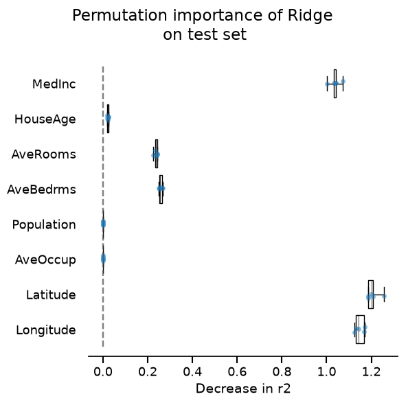
Scaled coefficients are one way to rank features. Another is permutation importance on held-out data: shuffle one column at a time and measure how much the score drops. That answers questions such as “which features did the model rely on most?” and works for nonlinear models as well. Present it as an alternative to scaled coefficients when you care about predictive reliance rather than a linear effect size.

Correlated features can distort both coefficient rankings and permutation importance (credit is shared or shifted between partners). See the SKD008 example and scikit-learn’s note on misleading values on strongly correlated features.

display = report.inspection.permutation_importance(
    seed=42,
    n_repeats=5,
)

display.frame()

	data_source	metric	feature	value_mean	value_std
0	test	r2	MedInc	1.038369	0.025849
1	test	r2	HouseAge	0.022603	0.002785
2	test	r2	AveRooms	0.236201	0.007711
3	test	r2	AveBedrms	0.257610	0.007691
4	test	r2	Population	0.000002	0.000039
5	test	r2	AveOccup	0.001057	0.000244
6	test	r2	Latitude	1.207360	0.028557
7	test	r2	Longitude	1.147209	0.020633

display.plot()

<Figure size 611.111x600 with 1 Axes>

Conclusion

SKD006 is a reminder to be careful when interpreting coefficients of linear models. When features are on different scales, linear coefficients mix feature importance with feature magnitude; when features are standardized, coefficients are comparable but no longer in original units.

Unscaled coefficients remain useful when the question is “if I change this feature by this much in its own units, how much does the prediction change?” Choose standardization, an effect-per-std rescaling, or a scale-invariant method such as permutation importance depending on the question you want to answer.