Store and retrieve reports on Skore Hub

This example shows how to use Project in hub mode: store reports remotely and inspect them. A key point is that summarize() returns a Summary, which is a pandas.DataFrame. In Jupyter you get an interactive widget, but you can always inspect and filter the summary as a DataFrame if you prefer.

Examples

To run this example and push in your own Skore Hub workspace and project, you can run this example with the following command:

WORKSPACE=<workspace> PROJECT=<project> python plot_skore_hub_project.py

In this gallery, we are going to push the different reports into a public workspace.

skore can communicate with Skore Hub which serves two main purposes: storing and retrieving any reports that you created and a user-friendly interface for you to explore and compare models.

First, we need to login to Skore Hub such that later we can push our reports to it.

from skore import login

login(mode="hub")

╭───────────────────────────────── Login to Skore Hub ─────────────────────────────────╮
│                                                                                      │
│                        Successfully logged in, using API key.                        │
│                                                                                      │
╰──────────────────────────────────────────────────────────────────────────────────────╯

To illustrate the integration with Skore Hub, we use a binary classification task where the goal is to predict whether a patient has a tumor or not.

import numpy as np
import skrub
from sklearn.datasets import load_breast_cancer

X, y = load_breast_cancer(return_X_y=True, as_frame=True)
labels = np.array(["no tumor", "tumor"], dtype=object)
y = labels[y]
skrub.TableReport(X)

Please enable javascript

The skrub table reports need javascript to display correctly. If you are displaying a report in a Jupyter notebook and you see this message, you may need to re-execute the cell or to trust the notebook (button on the top right or "File > Trust notebook").

Store reports on Skore Hub

On this problem, we use a logistic regression classifier with skrub’s tabular_pipeline() to preprocess the data if needed.

To send several reports to Skore Hub, we send models with different regularization parameters.

from numpy import logspace
from sklearn.linear_model import LogisticRegression
from skore import Project, evaluate

project = Project(f"{WORKSPACE}/{PROJECT}", mode="hub")

for regularization in logspace(-3, 3, 5):
    project.put(
        f"lr-regularization-{regularization:.1e}",
        evaluate(
            skrub.tabular_pipeline(LogisticRegression(C=regularization)),
            X,
            y,
            splitter=0.2,
            pos_label="tumor",
        ),
    )

  Putting lr-regularization-1.0e-03 0:00:35
Consult your report at
https://skore.probabl.ai/skore/example-skore-hub-project-dev/estimators/8701


  Putting lr-regularization-3.2e-02 0:00:35
Consult your report at
https://skore.probabl.ai/skore/example-skore-hub-project-dev/estimators/8702


  Putting lr-regularization-1.0e+00 0:00:37
Consult your report at
https://skore.probabl.ai/skore/example-skore-hub-project-dev/estimators/8703


  Putting lr-regularization-3.2e+01 0:00:35
Consult your report at
https://skore.probabl.ai/skore/example-skore-hub-project-dev/estimators/8704


  Putting lr-regularization-1.0e+03 0:00:35
Consult your report at
https://skore.probabl.ai/skore/example-skore-hub-project-dev/estimators/8705

Retrieve report stored on Skore Hub

Retrieving a report on Skore Hub is similar to retrieving a report in local mode.

summarize() returns a Summary, which subclasses pandas.DataFrame. In a Jupyter environment it renders an interactive parallel-coordinates widget by default.

summary = project.summarize()

To see the normal DataFrame table instead of the widget (e.g. in scripts or when you prefer the table), wrap the summary in pandas.DataFrame:

import pandas as pd

pandas_summary = pd.DataFrame(summary)
pandas_summary

		key	date	learner	ml_task	report_type	dataset	rmse	log_loss	roc_auc	fit_time	predict_time	rmse_mean	log_loss_mean	roc_auc_mean	fit_time_mean	predict_time_mean
	id
0	skore:report:estimator:8701	lr-regularization-1.0e-03	2026-04-29T16:07:11.000776+00:00	LogisticRegression	binary-classification	estimator	7887e234e3f622242e475e3da0cb5837	None	0.406397	0.987298	0.055146	0.034120	None	None	None	None	None
1	skore:report:estimator:8702	lr-regularization-3.2e-02	2026-04-29T16:07:46.872929+00:00	LogisticRegression	binary-classification	estimator	7887e234e3f622242e475e3da0cb5837	None	0.137499	0.995237	0.055377	0.033355	None	None	None	None	None
2	skore:report:estimator:8703	lr-regularization-1.0e+00	2026-04-29T16:08:24.393737+00:00	LogisticRegression	binary-classification	estimator	7887e234e3f622242e475e3da0cb5837	None	0.080457	0.995554	0.054876	0.032621	None	None	None	None	None
3	skore:report:estimator:8704	lr-regularization-3.2e+01	2026-04-29T16:09:00.004222+00:00	LogisticRegression	binary-classification	estimator	7887e234e3f622242e475e3da0cb5837	None	0.127249	0.992061	0.057464	0.032930	None	None	None	None	None
4	skore:report:estimator:8705	lr-regularization-1.0e+03	2026-04-29T16:09:35.496019+00:00	LogisticRegression	binary-classification	estimator	7887e234e3f622242e475e3da0cb5837	None	0.249399	0.990156	0.059721	0.033125	None	None	None	None	None

Basically, our summary contains metadata related to various information that we need to quickly help filtering the reports.

summary.info()

<class 'skore._project._summary.Summary'>
MultiIndex: 5 entries, (0, 'skore:report:estimator:8701') to (4, 'skore:report:estimator:8705')
Data columns (total 16 columns):
 #   Column             Non-Null Count  Dtype
---  ------             --------------  -----
 0   key                5 non-null      object
 1   date               5 non-null      object
 2   learner            5 non-null      category
 3   ml_task            5 non-null      object
 4   report_type        5 non-null      object
 5   dataset            5 non-null      object
 6   rmse               0 non-null      object
 7   log_loss           5 non-null      float64
 8   roc_auc            5 non-null      float64
 9   fit_time           5 non-null      float64
 10  predict_time       5 non-null      float64
 11  rmse_mean          0 non-null      object
 12  log_loss_mean      0 non-null      object
 13  roc_auc_mean       0 non-null      object
 14  fit_time_mean      0 non-null      object
 15  predict_time_mean  0 non-null      object
dtypes: category(1), float64(4), object(11)
memory usage: 1.1+ KB

Filter reports by metric (e.g. keep only those above a given accuracy) and work with the result as a table.

summary.query("log_loss < 0.2")["key"].tolist()

['lr-regularization-3.2e-02', 'lr-regularization-1.0e+00', 'lr-regularization-3.2e+01']

Use reports() to load the corresponding reports from the project (optionally after filtering the summary).

reports = summary.query("log_loss < 0.2").reports(return_as="comparison")
len(reports.reports_)

3

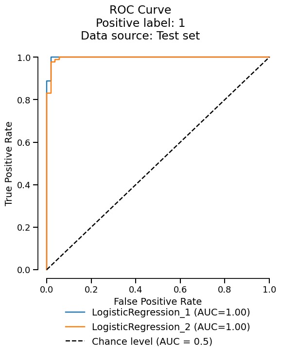
Since we got a ComparisonReport, we can use the metrics accessor to summarize the metrics across the reports.

reports.metrics.summarize().frame()

Estimator	LogisticRegression_1	LogisticRegression_2	LogisticRegression_3
Metric
Accuracy	0.956140	0.964912	0.947368
Precision	0.930556	0.970149	0.955224
Recall	1.000000	0.970149	0.955224
ROC AUC	0.995237	0.995554	0.992061
Log loss	0.137499	0.080457	0.127249
Brier score	0.035253	0.025149	0.029948
Fit time (s)	0.055377	0.054876	0.057464
Predict time (s)	0.033313	0.032726	0.032974

_ = reports.metrics.roc().plot(subplot_by=None)

Conclusion

Skore Hub provides a user-friendly interface for you to explore and compare models. You can easily store reports created using Skore.