Skore: getting started

This guide illustrates how to use skore through a complete machine learning workflow for binary classification:

1. Set up a proper experiment with training and test data

2. Develop and evaluate multiple models using cross-validation

3. Compare models to select the best one

4. Validate the final model on held-out data

5. Track and organize your machine learning results

Throughout this guide, we will see how skore helps you:

• Avoid common pitfalls with smart diagnostics

• Quickly get rich insights into model performance

• Organize and track your experiments

Setting up our binary classification problem

Let’s start by loading the German credit dataset, a classic binary classification problem where we predict the customer’s credit risk (“good” or “bad”).

This dataset contains various features about credit applicants, including personal information, credit history, and loan details.

import pandas as pd
import skore
from sklearn.datasets import fetch_openml
from skrub import TableReport

german_credit = fetch_openml(data_id=31, as_frame=True, parser="pandas")
X, y = german_credit.data, german_credit.target
TableReport(german_credit.frame)

Please enable javascript

The skrub table reports need javascript to display correctly. If you are displaying a report in a Jupyter notebook and you see this message, you may need to re-execute the cell or to trust the notebook (button on the top right or "File > Trust notebook").

Creating our experiment and held-out sets

We will use skore’s enhanced train_test_split() function to create our experiment set and a left-out test set. The experiment set will be used for model development and cross-validation, while the left-out set will only be used at the end to validate our final model.

Unlike scikit-learn’s train_test_split(), skore’s version provides helpful diagnostics about potential issues with your data split, such as class imbalance.

X_experiment, X_holdout, y_experiment, y_holdout = skore.train_test_split(
    X, y, random_state=42
)

╭────────────────────── HighClassImbalanceTooFewExamplesWarning ───────────────────────╮
│ It seems that you have a classification problem with at least one class with fewer   │
│ than 100 examples in the test set. In this case, using train_test_split may not be a │
│ good idea because of high variability in the scores obtained on the test set. We     │
│ suggest three options to tackle this challenge: you can increase test_size, collect  │
│ more data, or use skore's CrossValidationReport with the `splitter` parameter of     │
│ your choice.                                                                         │
╰──────────────────────────────────────────────────────────────────────────────────────╯
╭───────────────────────────────── ShuffleTrueWarning ─────────────────────────────────╮
│ We detected that the `shuffle` parameter is set to `True` either explicitly or from  │
│ its default value. In case of time-ordered events (even if they are independent),    │
│ this will result in inflated model performance evaluation because natural drift will │
│ not be taken into account. We recommend setting the shuffle parameter to `False` in  │
│ order to ensure the evaluation process is really representative of your production   │
│ release process.                                                                     │
╰──────────────────────────────────────────────────────────────────────────────────────╯

skore tells us we have class-imbalance issues with our data, which we confirm with the TableReport above by clicking on the “class” column and looking at the class distribution: there are only 300 examples where the target is “bad”. The second warning concerns time-ordered data, but our data does not contain time-ordered columns so we can safely ignore it.

Model development with cross-validation

We will investigate two different families of models using cross-validation.

1. A LogisticRegression which is a linear model

2. A RandomForestClassifier which is an ensemble of decision trees.

In both cases, we rely on skrub.tabular_pipeline() to choose the proper preprocessing depending on the kind of model.

Cross-validation is necessary to get a more reliable estimate of model performance. skore makes it easy through skore.CrossValidationReport.

Model no. 1: Linear regression with preprocessing

Our first model will be a linear model, with automatic preprocessing of non-numeric data. Under the hood, skrub’s TableVectorizer will adapt the preprocessing based on our choice to use a linear model.

from sklearn.linear_model import LogisticRegression
from skrub import tabular_pipeline

simple_model = tabular_pipeline(LogisticRegression())
simple_model

Pipeline(steps=[('tablevectorizer',
                 TableVectorizer(datetime=DatetimeEncoder(periodic_encoding='spline'))),
                ('simpleimputer', SimpleImputer(add_indicator=True)),
                ('squashingscaler', SquashingScaler(max_absolute_value=5)),
                ('logisticregression', LogisticRegression())])

In a Jupyter environment, please rerun this cell to show the HTML representation or trust the notebook.
On GitHub, the HTML representation is unable to render, please try loading this page with nbviewer.org.

We now cross-validate the model with CrossValidationReport.

from skore import CrossValidationReport

simple_cv_report = CrossValidationReport(
    simple_model,
    X=X_experiment,
    y=y_experiment,
    pos_label="good",
    splitter=5,
)

Skore reports allow us to structure the statistical information we look for when experimenting with predictive models. First, the help() method shows us all its available methods and attributes, with the knowledge that our model was trained for classification:

simple_cv_report.help()

╭─────────────────── Tools to diagnose estimator LogisticRegression ───────────────────╮
│ CrossValidationReport                                                                │
│ ├── .data                                                                            │
│ │   └── .analyze(...)                  - Plot dataset statistics.                    │
│ ├── .metrics                                                                         │
│ │   ├── .accuracy(...)         (↗︎)     - Compute the accuracy score.                 │
│ │   ├── .brier_score(...)      (↘︎)     - Compute the Brier score.                    │
│ │   ├── .confusion_matrix(...)         - Plot the confusion matrix.                  │
│ │   ├── .log_loss(...)         (↘︎)     - Compute the log loss.                       │
│ │   ├── .precision(...)        (↗︎)     - Compute the precision score.                │
│ │   ├── .precision_recall(...)         - Plot the precision-recall curve.            │
│ │   ├── .recall(...)           (↗︎)     - Compute the recall score.                   │
│ │   ├── .roc(...)                      - Plot the ROC curve.                         │
│ │   ├── .roc_auc(...)          (↗︎)     - Compute the ROC AUC score.                  │
│ │   ├── .timings(...)                  - Get all measured processing times related   │
│ │   │   to the estimator.                                                            │
│ │   ├── .custom_metric(...)            - Compute a custom metric.                    │
│ │   └── .summarize(...)                - Report a set of metrics for our estimator.  │
│ ├── .inspection                                                                      │
│ │   └── .coefficients(...)             - Retrieve the coefficients across splits,    │
│ │       including the intercept.                                                     │
│ ├── .cache_predictions(...)            - Cache the predictions for sub-estimators    │
│ │   reports.                                                                         │
│ ├── .clear_cache(...)                  - Clear the cache.                            │
│ ├── .create_estimator_report(...)      - Create an estimator report from the         │
│ │   cross-validation report.                                                         │
│ ├── .get_predictions(...)              - Get estimator's predictions.                │
│ └── Attributes                                                                       │
│     ├── .X                             - The data to fit                             │
│     ├── .y                             - The target variable to try to predict in    │
│     │   the case of supervised learning                                              │
│     ├── .estimator                     - Estimator to make the cross-validation      │
│     │   report from                                                                  │
│     ├── .estimator_                    - The cloned or copied estimator              │
│     ├── .estimator_name_               - The name of the estimator                   │
│     ├── .estimator_reports_            - The estimator reports for each split        │
│     ├── .ml_task                       - No description available                    │
│     ├── .n_jobs                        - Number of jobs to run in parallel           │
│     ├── .pos_label                     - For binary classification, the positive     │
│     │   class                                                                        │
│     ├── .split_indices                 - No description available                    │
│     └── .splitter                      - Determines the cross-validation splitting   │
│         strategy                                                                     │
│                                                                                      │
│                                                                                      │
│ Legend:                                                                              │
│ (↗︎) higher is better (↘︎) lower is better                                             │
╰──────────────────────────────────────────────────────────────────────────────────────╯

For example, we can examine the training data, which excludes the held-out data:

simple_cv_report.data.analyze()

Please enable javascript

The skrub table reports need javascript to display correctly. If you are displaying a report in a Jupyter notebook and you see this message, you may need to re-execute the cell or to trust the notebook (button on the top right or "File > Trust notebook").

But we can also quickly get an overview of the performance of our model, using summarize():

simple_metrics = simple_cv_report.metrics.summarize(favorability=True)
simple_metrics.frame()

	LogisticRegression		Favorability
	mean	std
Metric
Accuracy	0.729333	0.050903	(↗︎)
Precision	0.785632	0.034982	(↗︎)
Recall	0.840934	0.050696	(↗︎)
ROC AUC	0.750335	0.056447	(↗︎)
Brier score	0.184294	0.026786	(↘︎)
Fit time (s)	0.112525	0.009894	(↘︎)
Predict time (s)	0.054957	0.001311	(↘︎)

Note

favorability=True adds a column showing whether higher or lower metric values are better.

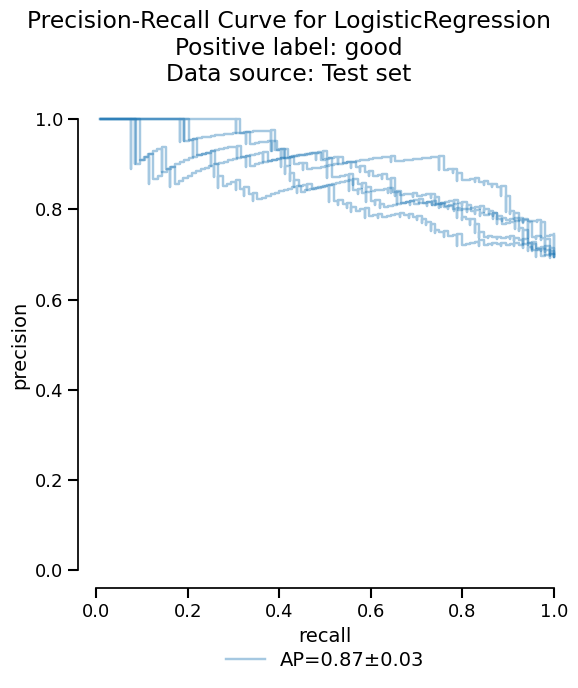
In addition to the summary of metrics, skore provides more advanced statistical information such as the precision-recall curve:

precision_recall = simple_cv_report.metrics.precision_recall()
precision_recall.help()

╭─────────────────────────── PrecisionRecallCurveDisplay  ───────────────────────────╮
│ display                                                                            │
│ ├──  Attributes                                                                    │
│ └── Methods                                                                        │
│     ├── .frame(...) - Get the data used to create the precision-recall curve plot. │
│     ├── .plot(...) - Plot visualization.                                           │
│     └── .set_style(...) - Set the style parameters for the display.                │
╰────────────────────────────────────────────────────────────────────────────────────╯

Note

The output of precision_recall() is a Display object. This is a common pattern in skore which allows us to access the information in several ways.

We can visualize the critical information as a plot, with only a few lines of code:

precision_recall.plot()

Or we can access the raw information as a dataframe if additional analysis is needed:

precision_recall.frame()

	split	threshold	precision	recall
0	0	0.110277	0.700000	1.000000
1	0	0.215387	0.744681	1.000000
2	0	0.238563	0.742857	0.990476
3	0	0.248819	0.741007	0.980952
4	0	0.273961	0.739130	0.971429
...	...	...	...	...
660	4	0.982595	1.000000	0.048077
661	4	0.988545	1.000000	0.038462
662	4	0.989817	1.000000	0.028846
663	4	0.994946	1.000000	0.019231
664	4	0.995636	1.000000	0.009615

665 rows × 4 columns

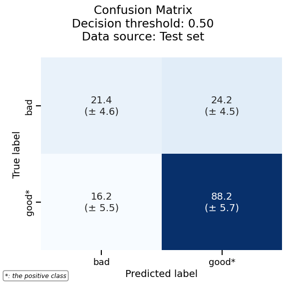
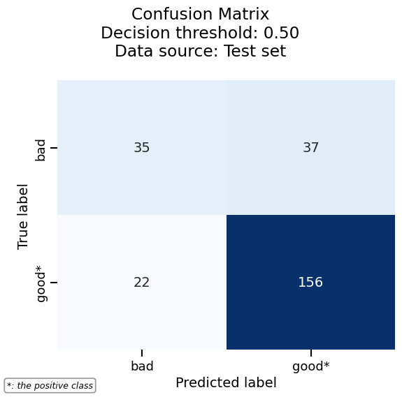
As another example, we can plot the confusion matrix with the same consistent API:

confusion_matrix = simple_cv_report.metrics.confusion_matrix()
confusion_matrix.plot()

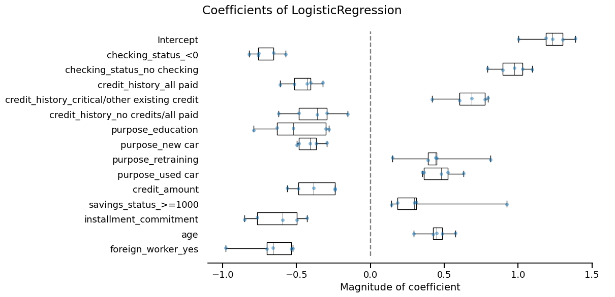
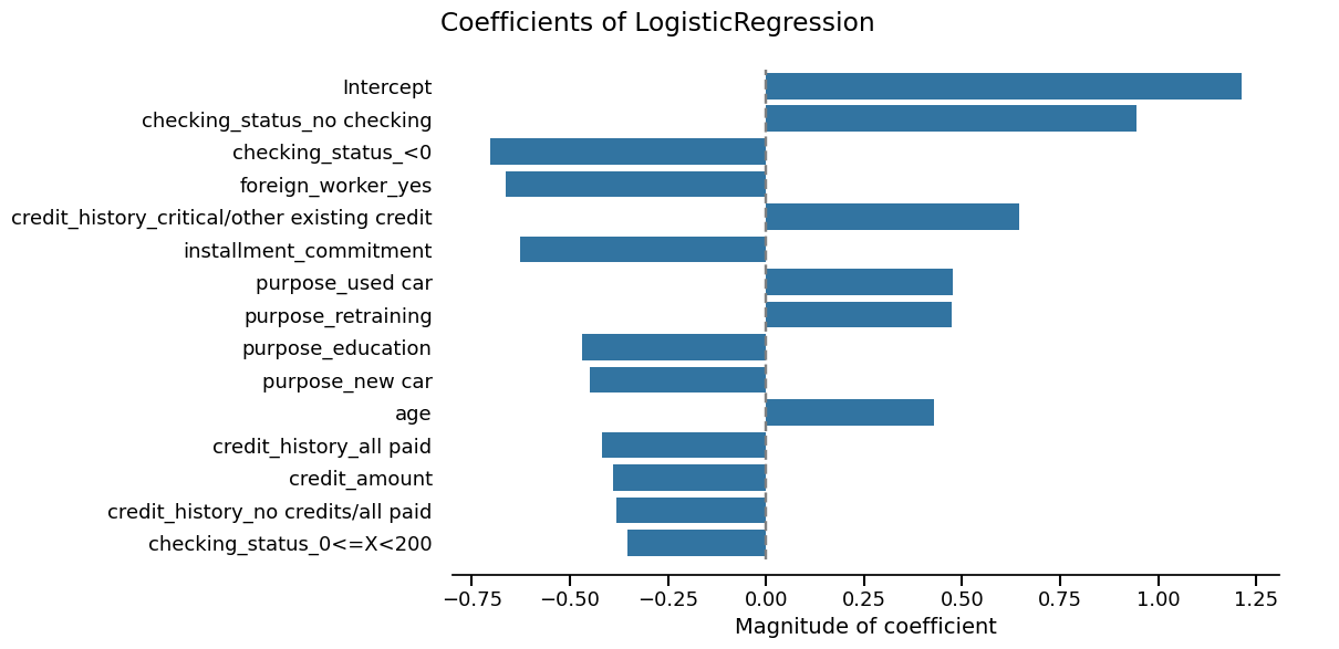
Skore also provides utilities to inspect models. Since our model is a linear model, we can study the importance that it gives to each feature:

coefficients = simple_cv_report.inspection.coefficients()
coefficients.frame()

	split	feature	coefficients
0	0	Intercept	1.232482
1	0	checking_status_0<=X<200	-0.322232
2	0	checking_status_<0	-0.572662
3	0	checking_status_>=200	0.196627
4	0	checking_status_no checking	0.791377
...	...	...	...
295	4	job_unemp/unskilled non res	0.272749
296	4	job_unskilled resident	0.118356
297	4	num_dependents	-0.112250
298	4	own_telephone_yes	0.319237
299	4	foreign_worker_yes	-0.660103

300 rows × 3 columns

coefficients.plot(select_k=15)

Model no. 2: Random forest

Now, we cross-validate a more advanced model using RandomForestClassifier. Again, we rely on tabular_pipeline() to perform the appropriate preprocessing to use with this model.

from sklearn.ensemble import RandomForestClassifier

advanced_model = tabular_pipeline(RandomForestClassifier(random_state=0))
advanced_model

Pipeline(steps=[('tablevectorizer',
                 TableVectorizer(low_cardinality=OrdinalEncoder(handle_unknown='use_encoded_value',
                                                                unknown_value=-1))),
                ('randomforestclassifier',
                 RandomForestClassifier(random_state=0))])

In a Jupyter environment, please rerun this cell to show the HTML representation or trust the notebook.
On GitHub, the HTML representation is unable to render, please try loading this page with nbviewer.org.

advanced_cv_report = CrossValidationReport(
    advanced_model, X=X_experiment, y=y_experiment, pos_label="good"
)

We will now compare this new model with the previous one.

Comparing our models

Now that we have our two models, we need to decide which one should go into production. We can compare them with a skore.ComparisonReport.

from skore import ComparisonReport

comparison = ComparisonReport(
    {
        "Simple Linear Model": simple_cv_report,
        "Advanced Pipeline": advanced_cv_report,
    },
)

This report follows the same API as CrossValidationReport:

comparison.help()

╭──────────────────────────── Tools to compare estimators ─────────────────────────────╮
│ ComparisonReport                                                                     │
│ ├── .metrics                                                                         │
│ │   ├── .accuracy(...)         (↗︎)     - Compute the accuracy score.                 │
│ │   ├── .brier_score(...)      (↘︎)     - Compute the Brier score.                    │
│ │   ├── .confusion_matrix(...)         - Plot the confusion matrix.                  │
│ │   ├── .log_loss(...)         (↘︎)     - Compute the log loss.                       │
│ │   ├── .precision(...)        (↗︎)     - Compute the precision score.                │
│ │   ├── .precision_recall(...)         - Plot the precision-recall curve.            │
│ │   ├── .recall(...)           (↗︎)     - Compute the recall score.                   │
│ │   ├── .roc(...)                      - Plot the ROC curve.                         │
│ │   ├── .roc_auc(...)          (↗︎)     - Compute the ROC AUC score.                  │
│ │   ├── .timings(...)                  - Get all measured processing times related   │
│ │   │   to the different estimators.                                                 │
│ │   ├── .custom_metric(...)            - Compute a custom metric.                    │
│ │   └── .summarize(...)                - Report a set of metrics for the estimators. │
│ ├── .inspection                                                                      │
│ ├── .cache_predictions(...)            - Cache the predictions for sub-estimators    │
│ │   reports.                                                                         │
│ ├── .clear_cache(...)                  - Clear the cache.                            │
│ ├── .create_estimator_report(...)      - Create an estimator report from one of the  │
│ │   reports in the comparison.                                                       │
│ ├── .get_predictions(...)              - Get predictions from the underlying         │
│ │   reports.                                                                         │
│ └── Attributes                                                                       │
│     ├── .n_jobs                        - Number of jobs to run in parallel           │
│     ├── .pos_label                     - No description available                    │
│     └── .reports_                      - The compared reports                        │
│                                                                                      │
│                                                                                      │
│ Legend:                                                                              │
│ (↗︎) higher is better (↘︎) lower is better                                             │
╰──────────────────────────────────────────────────────────────────────────────────────╯

We have access to the same tools to perform statistical analysis and compare both models:

comparison_metrics = comparison.metrics.summarize(favorability=True)
comparison_metrics.frame()

	mean		std		Favorability
Estimator	Simple Linear Model	Advanced Pipeline	Simple Linear Model	Advanced Pipeline
Metric
Accuracy	0.729333	0.745333	0.050903	0.032796	(↗︎)
Precision	0.785632	0.779443	0.034982	0.018644	(↗︎)
Recall	0.840934	0.885037	0.050696	0.053558	(↗︎)
ROC AUC	0.750335	0.773334	0.056447	0.034190	(↗︎)
Brier score	0.184294	0.169911	0.026786	0.010967	(↘︎)
Fit time (s)	0.112525	0.206632	0.009894	0.000750	(↘︎)
Predict time (s)	0.054957	0.050649	0.001311	0.000303	(↘︎)

comparison.metrics.precision_recall().plot()

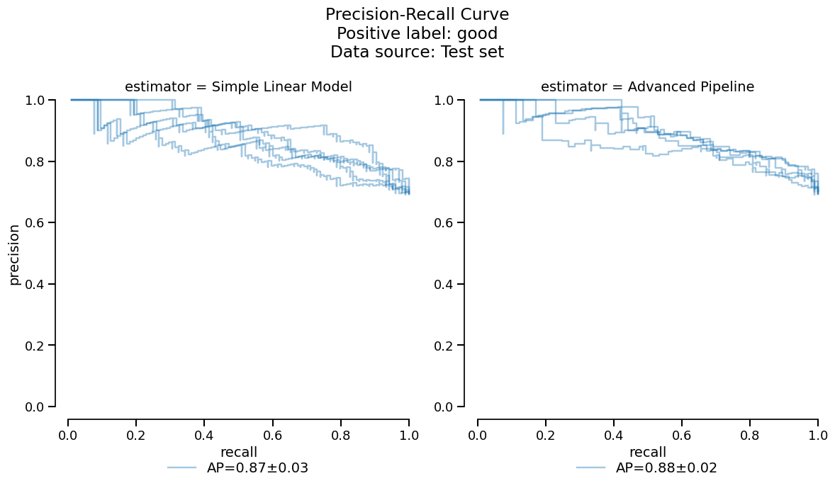
Based on the previous tables and plots, it seems that the RandomForestClassifier model has slightly better performance. For the purposes of this guide however, we make the arbitrary choice to deploy the linear model to make a comparison with the coefficients study shown earlier.

Final model evaluation on held-out data

Now that we have chosen to deploy the linear model, we will train it on the full experiment set and evaluate it on our held-out data: training on more data should help performance and we can also validate that our model generalizes well to new data. This can be done in one step with create_estimator_report().

final_report = comparison.create_estimator_report(
    name="Simple Linear Model", X_test=X_holdout, y_test=y_holdout
)

This returns a EstimatorReport which has a similar API to the other report classes:

final_metrics = final_report.metrics.summarize()
final_metrics.frame()

	LogisticRegression
Metric
Accuracy	0.764000
Precision	0.808290
Recall	0.876404
ROC AUC	0.809613
Brier score	0.153900
Fit time (s)	0.094362
Predict time (s)	0.055522

final_report.metrics.confusion_matrix().plot()

We can easily combine the results of the previous cross-validation together with the evaluation on the held-out dataset, since the two are accessible as dataframes. This way, we can check if our chosen model meets the expectations we set during the experiment phase.

pd.concat(
    [final_metrics.frame(), simple_cv_report.metrics.summarize().frame()],
    axis="columns",
)

	LogisticRegression	(LogisticRegression, mean)	(LogisticRegression, std)
Metric
Accuracy	0.764000	0.729333	0.050903
Precision	0.808290	0.785632	0.034982
Recall	0.876404	0.840934	0.050696
ROC AUC	0.809613	0.750335	0.056447
Brier score	0.153900	0.184294	0.026786
Fit time (s)	0.094362	0.112525	0.009894
Predict time (s)	0.055522	0.054957	0.001311

As expected, our final model gets better performance, likely thanks to the larger training set.

Our final sanity check is to compare the features considered most impactful between our final model and the cross-validation:

final_coefficients = final_report.inspection.coefficients()
final_top_15_features = final_coefficients.frame(select_k=15)["feature"]

simple_coefficients = simple_cv_report.inspection.coefficients()
cv_top_15_features = (
    simple_coefficients.frame(select_k=15)
    .groupby("feature", sort=False)
    .mean()
    .drop(columns="split")
    .reset_index()["feature"]
)

pd.concat(
    [final_top_15_features, cv_top_15_features], axis="columns", ignore_index=True
)

	0	1
0	Intercept	Intercept
1	checking_status_0<=X<200	checking_status_<0
2	checking_status_<0	checking_status_no checking
4	checking_status_no checking	credit_history_critical/other existing credit
6	credit_history_all paid	purpose_education
7	credit_history_critical/other existing credit	purpose_new car
10	credit_history_no credits/all paid	credit_amount
13	purpose_education	age
15	purpose_new car	NaN
19	purpose_retraining	NaN
20	purpose_used car	NaN
21	credit_amount	NaN
32	installment_commitment	NaN
45	age	NaN
59	foreign_worker_yes	NaN
3	NaN	credit_history_all paid
5	NaN	credit_history_no credits/all paid
8	NaN	purpose_retraining
9	NaN	purpose_used car
11	NaN	savings_status_>=1000
12	NaN	installment_commitment
14	NaN	foreign_worker_yes

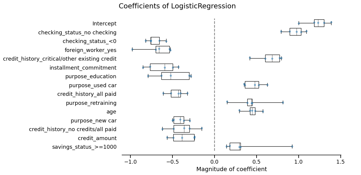
They seem very similar, so we are done!

Tracking our work with a skore Project

Now that we have completed our modeling workflow, we should store our models in a safe place for future work. Indeed, if this research notebook were modified, we would no longer be able to relate the current production model to the code that generated it.

We can use a skore.Project to keep track of our experiments. This makes it easy to organize, retrieve, and compare models over time.

Usually this would be done as you go along the model development, but in the interest of simplicity we kept this until the end.

We load or create a local project:

project = skore.Project("german_credit_classification")

We store our reports with descriptive keys:

project.put("simple_linear_model_cv", simple_cv_report)
project.put("advanced_pipeline_cv", advanced_cv_report)
project.put("final_model", final_report)

Now we can retrieve a summary of our stored reports:

summary = project.summarize()
# Uncomment the next line to display the widget in an interactive environment:
# summary

Note

Calling summary in a Jupyter notebook cell will show the following parallel coordinate plot to help you select models that you want to retrieve:

Each line represents a model, and we can select models by clicking on lines or dragging on metric axes to filter by performance.

In the screenshot, we selected only the cross-validation reports; this allows us to retrieve exactly those reports programmatically.

Supposing you selected “Cross-validation” in the “Report type” tab, if you now call reports(), you get only the CrossValidationReport objects, which you can directly put in the form of a ComparisonReport:

new_report = summary.reports(return_as="comparison")
new_report.help()

╭──────────────────────────── Tools to compare estimators ─────────────────────────────╮
│ ComparisonReport                                                                     │
│ ├── .metrics                                                                         │
│ │   ├── .accuracy(...)         (↗︎)     - Compute the accuracy score.                 │
│ │   ├── .brier_score(...)      (↘︎)     - Compute the Brier score.                    │
│ │   ├── .confusion_matrix(...)         - Plot the confusion matrix.                  │
│ │   ├── .log_loss(...)         (↘︎)     - Compute the log loss.                       │
│ │   ├── .precision(...)        (↗︎)     - Compute the precision score.                │
│ │   ├── .precision_recall(...)         - Plot the precision-recall curve.            │
│ │   ├── .recall(...)           (↗︎)     - Compute the recall score.                   │
│ │   ├── .roc(...)                      - Plot the ROC curve.                         │
│ │   ├── .roc_auc(...)          (↗︎)     - Compute the ROC AUC score.                  │
│ │   ├── .timings(...)                  - Get all measured processing times related   │
│ │   │   to the different estimators.                                                 │
│ │   ├── .custom_metric(...)            - Compute a custom metric.                    │
│ │   └── .summarize(...)                - Report a set of metrics for the estimators. │
│ ├── .inspection                                                                      │
│ ├── .cache_predictions(...)            - Cache the predictions for sub-estimators    │
│ │   reports.                                                                         │
│ ├── .clear_cache(...)                  - Clear the cache.                            │
│ ├── .create_estimator_report(...)      - Create an estimator report from one of the  │
│ │   reports in the comparison.                                                       │
│ ├── .get_predictions(...)              - Get predictions from the underlying         │
│ │   reports.                                                                         │
│ └── Attributes                                                                       │
│     ├── .n_jobs                        - Number of jobs to run in parallel           │
│     ├── .pos_label                     - No description available                    │
│     └── .reports_                      - The compared reports                        │
│                                                                                      │
│                                                                                      │
│ Legend:                                                                              │
│ (↗︎) higher is better (↘︎) lower is better                                             │
╰──────────────────────────────────────────────────────────────────────────────────────╯

Stay tuned!

This is only the beginning for skore. We welcome your feedback and ideas to make it the best tool for end-to-end data science.

Key benefits of using skore in your ML workflow:

• Standardized evaluation and comparison of models

• Rich visualizations and diagnostics

• Organized experiment tracking

• Seamless integration with scikit-learn

Feel free to join our community on Discord or create an issue.