Note
Go to the end to download the full example code.
EstimatorReport: Inspecting your models with the feature importance#
In this example, we tackle the California housing dataset where the goal is to perform
a regression task: predicting house prices based on features such as the number of
bedrooms, the geolocation, etc.
For that, we try out several families of models.
We evaluate these methods using evaluate() and the report’s metrics.
See also
As shown in EstimatorReport: Get insights from any scikit-learn estimator, the EstimatorReport has
a metrics() accessor that enables you to evaluate your
models and look at some scores that are automatically computed for you.
Here, we go beyond predictive performance, and inspect these models to better interpret
their behavior, by using feature importance.
Indeed, in practice, inspection can help spot some flaws in models: it is always
recommended to look “under the hood”.
For that, we use the unified inspection() accessor
of the EstimatorReport.
For linear models, we look at their coefficients.
For tree-based models, we inspect their mean decrease in impurity (MDI).
We can also inspect the permutation feature importance, that is model-agnostic.
Loading the dataset and performing some exploratory data analysis (EDA)#
Let us load the California housing dataset, which will enable us to perform a regression task about predicting house prices:
from skrub.datasets import fetch_california_housing

california_housing = fetch_california_housing()
dataset = california_housing.california_housing
X, y = california_housing.X, california_housing.y

dataset.head(2)
Downloading 'california_housing' from https://github.com/skrub-data/skrub-data-files/raw/refs/heads/main/california_housing.zip (attempt 1/3)
The documentation of the California housing dataset explains that the dataset
contains aggregated data regarding each district in California in 1990 and the target
(MedHouseVal) is the median house value for California districts,
expressed in hundreds of thousands of dollars ($100,000).
Note that there are some vacation resorts, with a large number of rooms and bedrooms.
See also
For more information about the California housing dataset, refer to scikit-learn MOOC’s page. Moreover, a more advanced modelling of this dataset is performed in this skops example.
Table report#
Let us perform some quick exploration on this dataset:
from skrub import TableReport

TableReport(dataset)
| MedInc | HouseAge | AveRooms | AveBedrms | Population | AveOccup | Latitude | Longitude | MedHouseVal | |
|---|---|---|---|---|---|---|---|---|---|
| 0 | 8.33 | 41.0 | 6.98 | 1.02 | 322. | 2.56 | 37.9 | -122. | 4.53 |
| 1 | 8.30 | 21.0 | 6.24 | 0.972 | 2.40e+03 | 2.11 | 37.9 | -122. | 3.58 |
| 2 | 7.26 | 52.0 | 8.29 | 1.07 | 496. | 2.80 | 37.9 | -122. | 3.52 |
| 3 | 5.64 | 52.0 | 5.82 | 1.07 | 558. | 2.55 | 37.9 | -122. | 3.41 |
| 4 | 3.85 | 52.0 | 6.28 | 1.08 | 565. | 2.18 | 37.9 | -122. | 3.42 |
| 20,635 | 1.56 | 25.0 | 5.05 | 1.13 | 845. | 2.56 | 39.5 | -121. | 0.781 |
| 20,636 | 2.56 | 18.0 | 6.11 | 1.32 | 356. | 3.12 | 39.5 | -121. | 0.771 |
| 20,637 | 1.70 | 17.0 | 5.21 | 1.12 | 1.01e+03 | 2.33 | 39.4 | -121. | 0.923 |
| 20,638 | 1.87 | 18.0 | 5.33 | 1.17 | 741. | 2.12 | 39.4 | -121. | 0.847 |
| 20,639 | 2.39 | 16.0 | 5.25 | 1.16 | 1.39e+03 | 2.62 | 39.4 | -121. | 0.894 |
MedInc
Float64DType- Null values
- 0 (0.0%)
- Unique values
-
12,928 (62.6%)
This column has a high cardinality (> 40).
- Mean ± Std
- 3.87 ± 1.90
- Median ± IQR
- 3.53 ± 2.18
- Min | Max
- 0.500 | 15.0
HouseAge
Float64DType- Null values
- 0 (0.0%)
- Unique values
-
52 (0.3%)
This column has a high cardinality (> 40).
- Mean ± Std
- 28.6 ± 12.6
- Median ± IQR
- 29.0 ± 19.0
- Min | Max
- 1.00 | 52.0
AveRooms
Float64DType- Null values
- 0 (0.0%)
- Unique values
-
19,392 (94.0%)
This column has a high cardinality (> 40).
- Mean ± Std
- 5.43 ± 2.47
- Median ± IQR
- 5.23 ± 1.61
- Min | Max
- 0.846 | 142.
AveBedrms
Float64DType- Null values
- 0 (0.0%)
- Unique values
-
14,233 (69.0%)
This column has a high cardinality (> 40).
- Mean ± Std
- 1.10 ± 0.474
- Median ± IQR
- 1.05 ± 0.0934
- Min | Max
- 0.333 | 34.1
Population
Float64DType- Null values
- 0 (0.0%)
- Unique values
-
3,888 (18.8%)
This column has a high cardinality (> 40).
- Mean ± Std
- 1.43e+03 ± 1.13e+03
- Median ± IQR
- 1.17e+03 ± 938.
- Min | Max
- 3.00 | 3.57e+04
AveOccup
Float64DType- Null values
- 0 (0.0%)
- Unique values
-
18,841 (91.3%)
This column has a high cardinality (> 40).
- Mean ± Std
- 3.07 ± 10.4
- Median ± IQR
- 2.82 ± 0.852
- Min | Max
- 0.692 | 1.24e+03
Latitude
Float64DType- Null values
- 0 (0.0%)
- Unique values
-
862 (4.2%)
This column has a high cardinality (> 40).
- Mean ± Std
- 35.6 ± 2.14
- Median ± IQR
- 34.3 ± 3.78
- Min | Max
- 32.5 | 42.0
Longitude
Float64DType- Null values
- 0 (0.0%)
- Unique values
-
844 (4.1%)
This column has a high cardinality (> 40).
- Mean ± Std
- -120. ± 2.00
- Median ± IQR
- -118. ± 3.79
- Min | Max
- -124. | -114.
MedHouseVal
Float64DType- Null values
- 0 (0.0%)
- Unique values
-
3,842 (18.6%)
This column has a high cardinality (> 40).
- Mean ± Std
- 2.07 ± 1.15
- Median ± IQR
- 1.80 ± 1.45
- Min | Max
- 0.150 | 5.00
No columns match the selected filter: . You can change the column filter in the dropdown menu above.
| Column | Column name | dtype | Is sorted | Null values | Unique values | Mean | Std | Min | Median | Max |
|---|---|---|---|---|---|---|---|---|---|---|
| 0 | MedInc | Float64DType | False | 0 (0.0%) | 12928 (62.6%) | 3.87 | 1.90 | 0.500 | 3.53 | 15.0 |
| 1 | HouseAge | Float64DType | False | 0 (0.0%) | 52 (0.3%) | 28.6 | 12.6 | 1.00 | 29.0 | 52.0 |
| 2 | AveRooms | Float64DType | False | 0 (0.0%) | 19392 (94.0%) | 5.43 | 2.47 | 0.846 | 5.23 | 142. |
| 3 | AveBedrms | Float64DType | False | 0 (0.0%) | 14233 (69.0%) | 1.10 | 0.474 | 0.333 | 1.05 | 34.1 |
| 4 | Population | Float64DType | False | 0 (0.0%) | 3888 (18.8%) | 1.43e+03 | 1.13e+03 | 3.00 | 1.17e+03 | 3.57e+04 |
| 5 | AveOccup | Float64DType | False | 0 (0.0%) | 18841 (91.3%) | 3.07 | 10.4 | 0.692 | 2.82 | 1.24e+03 |
| 6 | Latitude | Float64DType | False | 0 (0.0%) | 862 (4.2%) | 35.6 | 2.14 | 32.5 | 34.3 | 42.0 |
| 7 | Longitude | Float64DType | False | 0 (0.0%) | 844 (4.1%) | -120. | 2.00 | -124. | -118. | -114. |
| 8 | MedHouseVal | Float64DType | False | 0 (0.0%) | 3842 (18.6%) | 2.07 | 1.15 | 0.150 | 1.80 | 5.00 |
No columns match the selected filter: . You can change the column filter in the dropdown menu above.
MedInc
Float64DType- Null values
- 0 (0.0%)
- Unique values
-
12,928 (62.6%)
This column has a high cardinality (> 40).
- Mean ± Std
- 3.87 ± 1.90
- Median ± IQR
- 3.53 ± 2.18
- Min | Max
- 0.500 | 15.0
HouseAge
Float64DType- Null values
- 0 (0.0%)
- Unique values
-
52 (0.3%)
This column has a high cardinality (> 40).
- Mean ± Std
- 28.6 ± 12.6
- Median ± IQR
- 29.0 ± 19.0
- Min | Max
- 1.00 | 52.0
AveRooms
Float64DType- Null values
- 0 (0.0%)
- Unique values
-
19,392 (94.0%)
This column has a high cardinality (> 40).
- Mean ± Std
- 5.43 ± 2.47
- Median ± IQR
- 5.23 ± 1.61
- Min | Max
- 0.846 | 142.
AveBedrms
Float64DType- Null values
- 0 (0.0%)
- Unique values
-
14,233 (69.0%)
This column has a high cardinality (> 40).
- Mean ± Std
- 1.10 ± 0.474
- Median ± IQR
- 1.05 ± 0.0934
- Min | Max
- 0.333 | 34.1
Population
Float64DType- Null values
- 0 (0.0%)
- Unique values
-
3,888 (18.8%)
This column has a high cardinality (> 40).
- Mean ± Std
- 1.43e+03 ± 1.13e+03
- Median ± IQR
- 1.17e+03 ± 938.
- Min | Max
- 3.00 | 3.57e+04
AveOccup
Float64DType- Null values
- 0 (0.0%)
- Unique values
-
18,841 (91.3%)
This column has a high cardinality (> 40).
- Mean ± Std
- 3.07 ± 10.4
- Median ± IQR
- 2.82 ± 0.852
- Min | Max
- 0.692 | 1.24e+03
Latitude
Float64DType- Null values
- 0 (0.0%)
- Unique values
-
862 (4.2%)
This column has a high cardinality (> 40).
- Mean ± Std
- 35.6 ± 2.14
- Median ± IQR
- 34.3 ± 3.78
- Min | Max
- 32.5 | 42.0
Longitude
Float64DType- Null values
- 0 (0.0%)
- Unique values
-
844 (4.1%)
This column has a high cardinality (> 40).
- Mean ± Std
- -120. ± 2.00
- Median ± IQR
- -118. ± 3.79
- Min | Max
- -124. | -114.
MedHouseVal
Float64DType- Null values
- 0 (0.0%)
- Unique values
-
3,842 (18.6%)
This column has a high cardinality (> 40).
- Mean ± Std
- 2.07 ± 1.15
- Median ± IQR
- 1.80 ± 1.45
- Min | Max
- 0.150 | 5.00
No columns match the selected filter: . You can change the column filter in the dropdown menu above.
| Column 1 | Column 2 | Cramér's V | Pearson's Correlation |
|---|---|---|---|
| AveRooms | AveBedrms | 0.769 | 0.811 |
| Latitude | Longitude | 0.503 | -0.925 |
| Population | AveOccup | 0.316 | 0.111 |
| MedInc | MedHouseVal | 0.306 | 0.669 |
| MedInc | AveOccup | 0.267 | 0.0593 |
| MedInc | AveRooms | 0.194 | 0.354 |
| Longitude | MedHouseVal | 0.185 | -0.0431 |
| Latitude | MedHouseVal | 0.176 | -0.149 |
| HouseAge | Longitude | 0.173 | -0.0958 |
| AveBedrms | Longitude | 0.134 | 0.0123 |
| HouseAge | Latitude | 0.128 | -0.000739 |
| HouseAge | Population | 0.116 | -0.270 |
| AveRooms | MedHouseVal | 0.115 | 0.140 |
| AveRooms | Longitude | 0.0954 | -0.0316 |
| MedInc | Latitude | 0.0944 | -0.0783 |
| Population | Longitude | 0.0876 | 0.0923 |
| MedInc | Longitude | 0.0874 | -0.0110 |
| HouseAge | MedHouseVal | 0.0863 | 0.101 |
| HouseAge | AveRooms | 0.0858 | -0.186 |
| AveBedrms | Latitude | 0.0819 | 0.0769 |
| MedInc | HouseAge | 0.0771 | -0.121 |
| AveRooms | Latitude | 0.0757 | 0.117 |
| HouseAge | AveBedrms | 0.0745 | -0.117 |
| Population | MedHouseVal | 0.0653 | -0.0153 |
| MedInc | Population | 0.0642 | 0.0112 |
| HouseAge | AveOccup | 0.0566 | 0.0222 |
| Population | Latitude | 0.0491 | -0.0977 |
| AveBedrms | MedHouseVal | 0.0410 | -0.0613 |
| AveRooms | Population | 0.0401 | -0.0969 |
| AveOccup | Latitude | 0.0375 | 0.0173 |
| AveOccup | Longitude | 0.0375 | -0.0159 |
| MedInc | AveBedrms | 0.0349 | -0.0779 |
| AveOccup | MedHouseVal | 0.0333 | -0.0195 |
| AveBedrms | Population | 0.0233 | -0.0957 |
| AveRooms | AveOccup | 0.00558 | -0.0214 |
| AveBedrms | AveOccup | 0.00261 | -0.0147 |
Please enable javascript
The skrub table reports need javascript to display correctly. If you are displaying a report in a Jupyter notebook and you see this message, you may need to re-execute the cell or to trust the notebook (button on the top right or "File > Trust notebook").
From the table report, we can draw some key observations:
Looking at the Stats tab, all features are numerical and there are no missing values.
Looking at the Distributions tab, we can notice that some features seem to have some outliers:
MedInc,AveRooms,AveBedrms,Population, andAveOccup. The feature with the largest number of potential outliers isAveBedrms, probably corresponding to vacation resorts.Looking at the Associations tab, we observe that:
The target feature
MedHouseValis mostly associated withMedInc,Longitude, andLatitude. Indeed, intuitively, people with a large income would live in areas where the house prices are high. Moreover, we can expect some of these expensive areas to be close to one another.The association power between the target and these features is not super high, which would indicate that each single feature can not correctly predict the target. Given that
MedIncis associated withLongitudeand alsoLatitude, it might make sense to have some interactions between these features in our modelling: linear combinations might not be enough.
Target feature#
The target distribution has a long tail:
import matplotlib.pyplot as plt
import seaborn as sns

sns.histplot(data=dataset, x=y.name, bins=100)
plt.show(block=True)
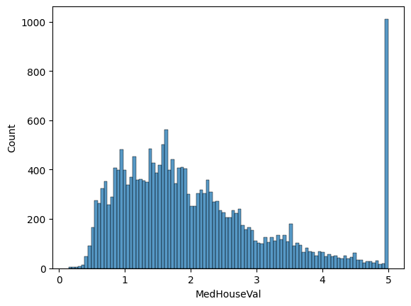
There seems to be a threshold-effect for high-valued houses: all houses with a price above $500,000 are given the value $500,000. We keep these clipped values in our data and will inspect how our models deal with them.
Now, as the median income MedInc is the feature with the highest association with
our target, let us assess how MedInc relates to MedHouseVal:
import pandas as pd
import plotly.express as px

X_y_plot = dataset.copy()
X_y_plot["MedInc_bins"] = pd.qcut(X_y_plot["MedInc"], q=5)
bin_order = X_y_plot["MedInc_bins"].cat.categories.sort_values()
fig = px.histogram(
    X_y_plot,
    x=y.name,
    color="MedInc_bins",
    category_orders={"MedInc_bins": bin_order},
)
fig
As could have been expected, a high salary often comes with a more expensive house. We can also notice the clipping effect of house prices for very high salaries.
Geospatial features#
From the table report, we noticed that the geospatial features Latitude and
Longitude were well associated with our target.
Hence, let us look into the coordinates of the districts in California, with regards
to the target feature, using a map:
def plot_map(df, color_feature):
    fig = px.scatter_map(
        df, lat="Latitude", lon="Longitude", color=color_feature, zoom=5, height=600
    )
    fig.update_layout(
        mapbox_style="open-street-map",
        mapbox_center={"lat": df["Latitude"].mean(), "lon": df["Longitude"].mean()},
        margin={"r": 0, "t": 0, "l": 0, "b": 0},
    )
    return fig
As could be expected, the price of the houses near the ocean is higher, especially around big cities like Los Angeles, San Francisco, and San Jose. Taking into account the coordinates in our modelling will be very important.
Linear models: coefficients#
For our regression task, we first use linear models. For feature importance, we inspect their coefficients.
Simple model#
Before trying any complex feature engineering, we start with a simple pipeline to
have a baseline of what a “good score” is (remember that all scores are relative).
We use a Ridge regression with feature scaling; and evaluate its performance using
evaluate() with splitter=0.2. This will evaluate the model on 20% of
the data after training on the remaining 80%, and report the results in an
EstimatorReport.
from sklearn.linear_model import Ridge
from sklearn.pipeline import make_pipeline
from sklearn.preprocessing import StandardScaler
from skore import evaluate

ridge_report = evaluate(make_pipeline(StandardScaler(), Ridge()), X, y, splitter=0.2)
ridge_report.metrics.summarize().frame()
From the report metrics, let us first explain the scores we have access to:
The coefficient of determination (
r2_score()), denoted as \(R^2\), which is a score. The best possible score is \(1\) and a constant model that always predicts the average value of the target would get a score of \(0\). Note that the score can be negative, as it could be worse than the average.The root mean squared error (
root_mean_squared_error()), abbreviated as RMSE, which is an error. It takes the square root of the mean squared error (MSE) so it is expressed in the same units as the target variable. The MSE measures the average squared difference between the predicted values and the actual values.
Here, the \(R^2\) seems quite poor, so some further preprocessing would be needed. This is done further down in this example.
Warning
Keep in mind that any observation drawn from inspecting the coefficients of this simple Ridge model is made on a model that performs quite poorly, hence must be treated with caution. Indeed, a poorly performing model does not capture the true underlying relationships in the data. A good practice would be to avoid inspecting models with poor performance. Here, we still inspect it, for demo purposes and because our model is not put into production!
Let us plot the prediction error:
_ = ridge_report.metrics.prediction_error().plot(kind="actual_vs_predicted")
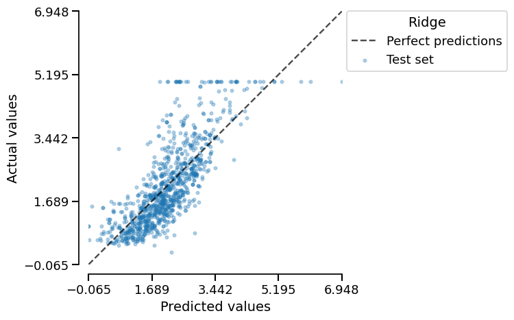
We can observe that the model has issues predicting large house prices, due to the clipping effect of the actual values.
Now, to inspect our model, let us use the
skore.EstimatorReport.inspection() accessor:
ridge_report.inspection.coefficients().frame()
Note
Beware that coefficients can be misleading when some features are correlated. For example, two coefficients can have large absolute values (so be considered important), but in the predictions, the sum of their contributions could cancel out (if they are highly correlated), so they would actually be unimportant.
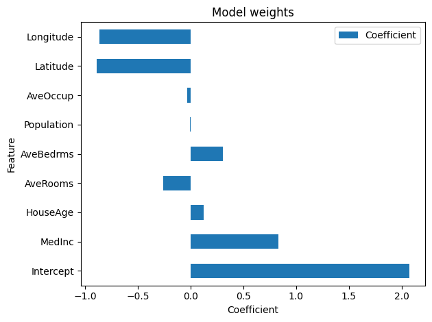
We can plot this pandas datafame:
_ = ridge_report.inspection.coefficients().plot()
Note
More generally, skore.EstimatorReport.inspection.coefficients() can
help you inspect the coefficients of all linear models.
We consider a linear model as defined in
scikit-learn’s documentation.
In short, we consider a “linear model” as a scikit-learn compatible estimator that
holds a coef_ attribute (after being fitted).
Since we have included scaling in the pipeline, the resulting coefficients are all on the same scale, making them directly comparable to each other. Without this scaling step, the coefficients in a linear model would be influenced by the original scale of the feature values, which would prevent meaningful comparisons between them.
See also
For more information about the importance of scaling, see scikit-learn’s example on Common pitfalls in the interpretation of coefficients of linear models.
Here, it appears that the MedInc, Latitude, and Longitude features are
the most important, with regards to the absolute value of other coefficients.
This finding is consistent with our previous observations from the Associations
tab of the table report.
However, due to the scaling, we can not interpret the coefficient values with regards to the original unit of the feature. Let us unscale the coefficients, without forgetting the intercept, so that the coefficients can be interpreted using the original units:
import numpy as np

# retrieve the mean and standard deviation used to standardize the feature values
feature_mean = ridge_report.estimator_[0].mean_
feature_std = ridge_report.estimator_[0].scale_


def unscale_coefficients(df, feature_mean, feature_std):
    df = df.set_index("feature")
    mask_intercept_column = df.index == "Intercept"
    # rescale the intercept
    df.loc[mask_intercept_column] = df.loc[mask_intercept_column] - np.sum(
        df.loc[~mask_intercept_column, "coefficient"] * feature_mean / feature_std
    )
    # rescale the other coefficients
    df.loc[~mask_intercept_column, "coefficient"] = (
        df.loc[~mask_intercept_column, "coefficient"] / feature_std
    )
    return df.reset_index()


df_ridge_report_coef_unscaled = unscale_coefficients(
    ridge_report.inspection.coefficients().frame(), feature_mean, feature_std
)
df_ridge_report_coef_unscaled
Now, we can interpret each coefficient values with regards to the original units.
We can interpret a coefficient as follows: according to our model, on average,
having one additional bedroom (a increase of \(1\) of AveBedrms),
with all other features being constant,
increases the predicted house value of \(0.62\) in $100,000, hence of $62,000.
Note that we have not dealt with any potential outlier in this iteration.
Warning
Recall that we are inspecting a model with poor performance, which is bad practice. Moreover, we must be cautious when trying to induce any causation effect (remember that correlation is not causation).
More complex model#
As previously mentioned, our simple Ridge model, although very easily interpretable with regards to the original units of the features, performs quite poorly. Now, we build a more complex model, with more feature engineering. We will see that this model will have a better score… but will be more difficult to interpret the coefficients with regards to the original features due to the complex feature engineering.
In our previous EDA, when plotting the geospatial data with regards to the house prices, we noticed that it is important to take into account the latitude and longitude features. Moreover, we also observed that the median income is well associated with the house prices. Hence, we will try a feature engineering that takes into account the interactions of the geospatial features with features such as the income, using polynomial features. The interactions are no longer simply linear as previously.
Let us build a model with some more complex feature engineering, and still use a Ridge regressor (linear model) at the end of the pipeline. In particular, we perform a K-means clustering on the geospatial features:
from sklearn.cluster import KMeans
from sklearn.compose import make_column_transformer
from sklearn.preprocessing import PolynomialFeatures, SplineTransformer

geo_columns = ["Latitude", "Longitude"]

preprocessor = make_column_transformer(
    (KMeans(n_clusters=10, random_state=0), geo_columns),
    remainder="passthrough",
)
engineered_ridge = make_pipeline(
    preprocessor,
    SplineTransformer(sparse_output=True),
    PolynomialFeatures(degree=2, interaction_only=True, include_bias=False),
    Ridge(),
)
engineered_ridge
Now, let us compute the metrics and compare it to our previous model using
the compare() function that returns a ComparisonReport:
from skore import compare

engineered_ridge_report = evaluate(engineered_ridge, X, y, splitter=0.2)
reports_to_compare = {
    "Vanilla Ridge": ridge_report,
    "Ridge w/ feature engineering": engineered_ridge_report,
}
comparator = compare(reports_to_compare)
comparator.metrics.summarize().frame()
We get a much better score! Let us plot the prediction error:
_ = engineered_ridge_report.metrics.prediction_error().plot(kind="actual_vs_predicted")
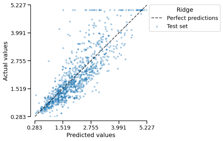
About the clipping issue, compared to the prediction error of our previous model
(ridge_report), our engineered_ridge_report model seems to produce predictions
that are not as large, so it seems that some interactions between features have
helped alleviate the clipping issue.
However, interpreting the features is harder: indeed, our complex feature engineering introduced a lot of features:
n_features_initial = ridge_report.X_train.shape[1]
print("Initial number of features:", n_features_initial)

# We slice the scikit-learn pipeline to extract the predictor, using -1 to access
# the last step:
n_features_engineered = engineered_ridge_report.estimator_[-1].n_features_in_
print("Number of features after feature engineering:", n_features_engineered)
Initial number of features: 8
Number of features after feature engineering: 6328
Let us display the 15 largest absolute coefficients:
engineered_ridge_report_coefficients = (
    engineered_ridge_report.inspection.coefficients()
    .frame()
    .set_index("feature")
    .sort_values(by="coefficient", key=abs, ascending=True)
    .tail(15)
)

engineered_ridge_report_coefficients.index = (
    engineered_ridge_report_coefficients.index.str.replace("remainder__", "")
)
engineered_ridge_report_coefficients.index = (
    engineered_ridge_report_coefficients.index.str.replace("kmeans__", "geospatial__")
)

engineered_ridge_report_coefficients.plot.barh(
    title="Model weights",
    xlabel="Coefficient",
    ylabel="Feature",
)
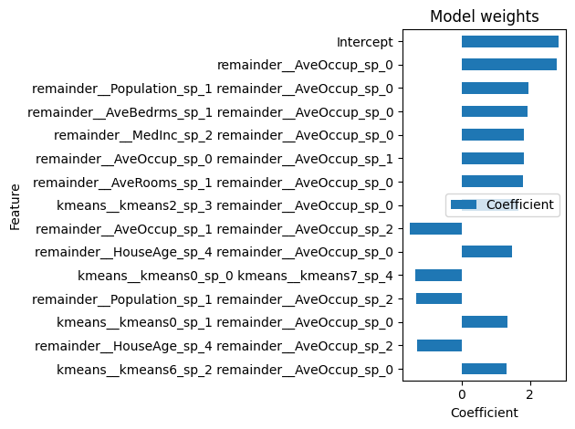
<Axes: title={'center': 'Model weights'}, xlabel='Coefficient', ylabel='Feature'>
We can observe that the most important features are interactions between features,
mostly based on AveOccup, that a simple linear model without feature engineering
could not have captured.
Indeed, the vanilla Ridge model did not consider AveOccup to be important.
As the engineered Ridge has a better score, perhaps the vanilla Ridge missed
something about AveOccup that seems to be key to predicting house prices.
Let us visualize how AveOccup interacts with MedHouseVal:
Finally, we can visualize the results of our K-means clustering (on the training set):
# getting the cluster labels
col_transformer = engineered_ridge_report.estimator_.named_steps["columntransformer"]
kmeans = col_transformer.named_transformers_["kmeans"]
clustering_labels = kmeans.labels_

# adding the cluster labels to our dataframe
X_train_plot = ridge_report.X_train.copy()
X_train_plot.insert(n_features_initial, "clustering_labels", clustering_labels)

# plotting the map
plot_map(X_train_plot, "clustering_labels")
Inspecting the prediction error at the sample level#
After feature importance, we now try to understand why our model performs badly on some samples, in order to iterate on our estimator pipeline and improve it.
We compute the prediction squared error at the sample level, named squared_error,
on the train and test sets:
def add_y_true_pred(model_report, split):
    """
    Concatenate the design matrix (`X`) with the actual targets (`y`)
    and predicted ones (`y_pred`) from a fitted skore EstimatorReport,
    either on the train or the test set.
    """

    if split == "train":
        y_split_true = model_report.y_train
        X_split = model_report.X_train.copy()
    elif split == "test":
        y_split_true = model_report.y_test
        X_split = model_report.X_test.copy()
    else:
        raise ValueError("split must be either `train`, or `test`")

    # adding a `split` feature
    X_split.insert(0, "split", split)

    # retrieving the predictions
    y_split_pred = model_report.get_predictions(
        data_source=split, response_method="predict"
    )

    # computing the squared error at the sample level
    squared_error_split = (y_split_true - y_split_pred) ** 2

    # adding the squared error to our dataframes
    X_split.insert(X_split.shape[1], "squared_error", squared_error_split)

    # adding the true values and the predictions
    X_y_split = X_split.copy()
    X_y_split.insert(X_y_split.shape[1], "y_true", y_split_true)
    X_y_split.insert(X_y_split.shape[1], "y_pred", y_split_pred)
    return X_y_split
X_y_train_plot = add_y_true_pred(engineered_ridge_report, "train")
X_y_test_plot = add_y_true_pred(engineered_ridge_report, "test")
X_y_plot = pd.concat([X_y_train_plot, X_y_test_plot])
X_y_plot.sample(10)
We visualize the distributions of the prediction errors on both train and test sets:
sns.histplot(data=X_y_plot, x="squared_error", hue="split", multiple="dodge", bins=30)
plt.title("Train and test sets")
plt.show(block=True)
Now, in order to assess which features might drive the prediction error, let us look
into the associations between the squared_error and the other features:
from skrub import column_associations

column_associations(X_y_plot).query(
    "left_column_name == 'squared_error' or right_column_name == 'squared_error'"
)
We observe that the AveOccup feature leads to large prediction errors: our model
is not able to deal well with that feature.
Hence, it might be worth it to dive deep into the AveOccup feature, for
example its outliers.
We observe that we have large prediction errors for districts near the coast and big cities:
threshold = X_y_plot["squared_error"].quantile(0.95)  # out of the train and test sets
plot_map(X_y_plot.query(f"squared_error > {threshold}"), "split")
Hence, it could make sense to engineer two new features: the distance to the coast and the distance to big cities.
Most of our very bad predictions underpredict the true value (y_true is more often
larger than y_pred):
# Create the scatter plot
fig = px.scatter(
    X_y_plot.query(f"squared_error > {threshold}"),
    x="y_pred",
    y="y_true",
    color="split",
)
# Add the diagonal line
fig.add_shape(
    type="line",
    x0=X_y_plot["y_pred"].min(),
    y0=X_y_plot["y_pred"].min(),
    x1=X_y_plot["y_pred"].max(),
    y1=X_y_plot["y_pred"].max(),
    line={"color": "black", "width": 2},
)
fig
Compromising on complexity#
Now, let us build a model with a more interpretable feature engineering, although
it might not perform as well.
For that, after the complex feature engineering, we perform some feature selection
using a SelectKBest, in order to reduce the
number of features.
from sklearn.feature_selection import SelectKBest, VarianceThreshold, f_regression
from sklearn.linear_model import RidgeCV

preprocessor = make_column_transformer(
    (KMeans(n_clusters=10, random_state=0), geo_columns),
    remainder="passthrough",
)
selectkbest_ridge = make_pipeline(
    preprocessor,
    SplineTransformer(sparse_output=True),
    PolynomialFeatures(degree=2, interaction_only=True, include_bias=False),
    VarianceThreshold(1e-8),
    SelectKBest(score_func=lambda X, y: f_regression(X, y, center=False), k=150),
    RidgeCV(np.logspace(-5, 5, num=100)),
)
Note
To keep the computation time of this example low, we did not tune
the hyperparameters of the predictive model. However, on a real use
case, it would be important to tune the model using
RandomizedSearchCV
and not just the RidgeCV.
Let us get the metrics for our model and compare it with our previous iterations:
selectk_ridge_report = evaluate(selectkbest_ridge, X, y, splitter=0.2)
reports_to_compare["Ridge w/ feature engineering and selection"] = selectk_ridge_report
comparator = compare(reports_to_compare)
comparator.metrics.summarize().frame()
We get a good score and much less features:
print("Initial number of features:", n_features_initial)
print("Number of features after feature engineering:", n_features_engineered)

n_features_selectk = selectk_ridge_report.estimator_[-1].n_features_in_
print(
    "Number of features after feature engineering using `SelectKBest`:",
    n_features_selectk,
)
Initial number of features: 8
Number of features after feature engineering: 6328
Number of features after feature engineering using `SelectKBest`: 150
According to the SelectKBest, the most important
features are the following:
selectk_features = selectk_ridge_report.estimator_[:-1].get_feature_names_out()
print(selectk_features)
['kmeans__kmeans3_sp_2' 'kmeans__kmeans3_sp_3' 'kmeans__kmeans9_sp_2'
 'remainder__MedInc_sp_2' 'remainder__MedInc_sp_3'
 'remainder__AveRooms_sp_0' 'remainder__AveRooms_sp_1'
 'remainder__AveRooms_sp_2' 'remainder__AveBedrms_sp_0'
 'remainder__AveBedrms_sp_1' 'remainder__AveBedrms_sp_2'
 'remainder__Population_sp_0' 'remainder__Population_sp_1'
 'remainder__Population_sp_2' 'remainder__AveOccup_sp_0'
 'remainder__AveOccup_sp_1' 'remainder__AveOccup_sp_2'
 'kmeans__kmeans3_sp_2 kmeans__kmeans3_sp_3'
 'kmeans__kmeans3_sp_2 kmeans__kmeans9_sp_2'
 'kmeans__kmeans3_sp_2 remainder__AveRooms_sp_0'
 'kmeans__kmeans3_sp_2 remainder__AveRooms_sp_1'
 'kmeans__kmeans3_sp_2 remainder__AveRooms_sp_2'
 'kmeans__kmeans3_sp_2 remainder__AveBedrms_sp_0'
 'kmeans__kmeans3_sp_2 remainder__AveBedrms_sp_1'
 'kmeans__kmeans3_sp_2 remainder__AveBedrms_sp_2'
 'kmeans__kmeans3_sp_2 remainder__Population_sp_0'
 'kmeans__kmeans3_sp_2 remainder__Population_sp_1'
 'kmeans__kmeans3_sp_2 remainder__Population_sp_2'
 'kmeans__kmeans3_sp_2 remainder__AveOccup_sp_0'
 'kmeans__kmeans3_sp_2 remainder__AveOccup_sp_1'
 'kmeans__kmeans3_sp_2 remainder__AveOccup_sp_2'
 'kmeans__kmeans3_sp_3 kmeans__kmeans8_sp_3'
 'kmeans__kmeans3_sp_3 kmeans__kmeans9_sp_2'
 'kmeans__kmeans3_sp_3 remainder__MedInc_sp_2'
 'kmeans__kmeans3_sp_3 remainder__MedInc_sp_3'
 'kmeans__kmeans3_sp_3 remainder__AveRooms_sp_0'
 'kmeans__kmeans3_sp_3 remainder__AveRooms_sp_1'
 'kmeans__kmeans3_sp_3 remainder__AveRooms_sp_2'
 'kmeans__kmeans3_sp_3 remainder__AveBedrms_sp_0'
 'kmeans__kmeans3_sp_3 remainder__AveBedrms_sp_1'
 'kmeans__kmeans3_sp_3 remainder__AveBedrms_sp_2'
 'kmeans__kmeans3_sp_3 remainder__Population_sp_0'
 'kmeans__kmeans3_sp_3 remainder__Population_sp_1'
 'kmeans__kmeans3_sp_3 remainder__Population_sp_2'
 'kmeans__kmeans3_sp_3 remainder__AveOccup_sp_0'
 'kmeans__kmeans3_sp_3 remainder__AveOccup_sp_1'
 'kmeans__kmeans3_sp_3 remainder__AveOccup_sp_2'
 'kmeans__kmeans9_sp_2 kmeans__kmeans9_sp_3'
 'kmeans__kmeans9_sp_2 remainder__MedInc_sp_3'
 'kmeans__kmeans9_sp_2 remainder__AveRooms_sp_0'
 'kmeans__kmeans9_sp_2 remainder__AveRooms_sp_1'
 'kmeans__kmeans9_sp_2 remainder__AveRooms_sp_2'
 'kmeans__kmeans9_sp_2 remainder__AveBedrms_sp_0'
 'kmeans__kmeans9_sp_2 remainder__AveBedrms_sp_1'
 'kmeans__kmeans9_sp_2 remainder__AveBedrms_sp_2'
 'kmeans__kmeans9_sp_2 remainder__Population_sp_0'
 'kmeans__kmeans9_sp_2 remainder__Population_sp_1'
 'kmeans__kmeans9_sp_2 remainder__Population_sp_2'
 'kmeans__kmeans9_sp_2 remainder__AveOccup_sp_0'
 'kmeans__kmeans9_sp_2 remainder__AveOccup_sp_1'
 'kmeans__kmeans9_sp_2 remainder__AveOccup_sp_2'
 'remainder__MedInc_sp_2 remainder__MedInc_sp_3'
 'remainder__MedInc_sp_2 remainder__AveRooms_sp_0'
 'remainder__MedInc_sp_2 remainder__AveRooms_sp_1'
 'remainder__MedInc_sp_2 remainder__AveRooms_sp_2'
 'remainder__MedInc_sp_2 remainder__AveBedrms_sp_0'
 'remainder__MedInc_sp_2 remainder__AveBedrms_sp_1'
 'remainder__MedInc_sp_2 remainder__AveBedrms_sp_2'
 'remainder__MedInc_sp_2 remainder__Population_sp_0'
 'remainder__MedInc_sp_2 remainder__Population_sp_1'
 'remainder__MedInc_sp_2 remainder__AveOccup_sp_0'
 'remainder__MedInc_sp_2 remainder__AveOccup_sp_1'
 'remainder__MedInc_sp_2 remainder__AveOccup_sp_2'
 'remainder__MedInc_sp_3 remainder__AveRooms_sp_0'
 'remainder__MedInc_sp_3 remainder__AveRooms_sp_1'
 'remainder__MedInc_sp_3 remainder__AveRooms_sp_2'
 'remainder__MedInc_sp_3 remainder__AveBedrms_sp_0'
 'remainder__MedInc_sp_3 remainder__AveBedrms_sp_1'
 'remainder__MedInc_sp_3 remainder__AveBedrms_sp_2'
 'remainder__MedInc_sp_3 remainder__Population_sp_0'
 'remainder__MedInc_sp_3 remainder__Population_sp_1'
 'remainder__MedInc_sp_3 remainder__AveOccup_sp_0'
 'remainder__MedInc_sp_3 remainder__AveOccup_sp_1'
 'remainder__MedInc_sp_3 remainder__AveOccup_sp_2'
 'remainder__AveRooms_sp_0 remainder__AveRooms_sp_1'
 'remainder__AveRooms_sp_0 remainder__AveRooms_sp_2'
 'remainder__AveRooms_sp_0 remainder__AveBedrms_sp_0'
 'remainder__AveRooms_sp_0 remainder__AveBedrms_sp_1'
 'remainder__AveRooms_sp_0 remainder__AveBedrms_sp_2'
 'remainder__AveRooms_sp_0 remainder__Population_sp_0'
 'remainder__AveRooms_sp_0 remainder__Population_sp_1'
 'remainder__AveRooms_sp_0 remainder__Population_sp_2'
 'remainder__AveRooms_sp_0 remainder__AveOccup_sp_0'
 'remainder__AveRooms_sp_0 remainder__AveOccup_sp_1'
 'remainder__AveRooms_sp_0 remainder__AveOccup_sp_2'
 'remainder__AveRooms_sp_1 remainder__AveRooms_sp_2'
 'remainder__AveRooms_sp_1 remainder__AveBedrms_sp_0'
 'remainder__AveRooms_sp_1 remainder__AveBedrms_sp_1'
 'remainder__AveRooms_sp_1 remainder__AveBedrms_sp_2'
 'remainder__AveRooms_sp_1 remainder__Population_sp_0'
 'remainder__AveRooms_sp_1 remainder__Population_sp_1'
 'remainder__AveRooms_sp_1 remainder__Population_sp_2'
 'remainder__AveRooms_sp_1 remainder__AveOccup_sp_0'
 'remainder__AveRooms_sp_1 remainder__AveOccup_sp_1'
 'remainder__AveRooms_sp_1 remainder__AveOccup_sp_2'
 'remainder__AveRooms_sp_2 remainder__AveBedrms_sp_0'
 'remainder__AveRooms_sp_2 remainder__AveBedrms_sp_1'
 'remainder__AveRooms_sp_2 remainder__AveBedrms_sp_2'
 'remainder__AveRooms_sp_2 remainder__Population_sp_0'
 'remainder__AveRooms_sp_2 remainder__Population_sp_1'
 'remainder__AveRooms_sp_2 remainder__Population_sp_2'
 'remainder__AveRooms_sp_2 remainder__AveOccup_sp_0'
 'remainder__AveRooms_sp_2 remainder__AveOccup_sp_1'
 'remainder__AveRooms_sp_2 remainder__AveOccup_sp_2'
 'remainder__AveBedrms_sp_0 remainder__AveBedrms_sp_1'
 'remainder__AveBedrms_sp_0 remainder__AveBedrms_sp_2'
 'remainder__AveBedrms_sp_0 remainder__Population_sp_0'
 'remainder__AveBedrms_sp_0 remainder__Population_sp_1'
 'remainder__AveBedrms_sp_0 remainder__Population_sp_2'
 'remainder__AveBedrms_sp_0 remainder__AveOccup_sp_0'
 'remainder__AveBedrms_sp_0 remainder__AveOccup_sp_1'
 'remainder__AveBedrms_sp_0 remainder__AveOccup_sp_2'
 'remainder__AveBedrms_sp_1 remainder__AveBedrms_sp_2'
 'remainder__AveBedrms_sp_1 remainder__Population_sp_0'
 'remainder__AveBedrms_sp_1 remainder__Population_sp_1'
 'remainder__AveBedrms_sp_1 remainder__Population_sp_2'
 'remainder__AveBedrms_sp_1 remainder__AveOccup_sp_0'
 'remainder__AveBedrms_sp_1 remainder__AveOccup_sp_1'
 'remainder__AveBedrms_sp_1 remainder__AveOccup_sp_2'
 'remainder__AveBedrms_sp_2 remainder__Population_sp_0'
 'remainder__AveBedrms_sp_2 remainder__Population_sp_1'
 'remainder__AveBedrms_sp_2 remainder__Population_sp_2'
 'remainder__AveBedrms_sp_2 remainder__AveOccup_sp_0'
 'remainder__AveBedrms_sp_2 remainder__AveOccup_sp_1'
 'remainder__AveBedrms_sp_2 remainder__AveOccup_sp_2'
 'remainder__Population_sp_0 remainder__Population_sp_1'
 'remainder__Population_sp_0 remainder__Population_sp_2'
 'remainder__Population_sp_0 remainder__AveOccup_sp_0'
 'remainder__Population_sp_0 remainder__AveOccup_sp_1'
 'remainder__Population_sp_0 remainder__AveOccup_sp_2'
 'remainder__Population_sp_1 remainder__Population_sp_2'
 'remainder__Population_sp_1 remainder__AveOccup_sp_0'
 'remainder__Population_sp_1 remainder__AveOccup_sp_1'
 'remainder__Population_sp_1 remainder__AveOccup_sp_2'
 'remainder__Population_sp_2 remainder__AveOccup_sp_0'
 'remainder__Population_sp_2 remainder__AveOccup_sp_1'
 'remainder__Population_sp_2 remainder__AveOccup_sp_2'
 'remainder__AveOccup_sp_0 remainder__AveOccup_sp_1'
 'remainder__AveOccup_sp_0 remainder__AveOccup_sp_2'
 'remainder__AveOccup_sp_1 remainder__AveOccup_sp_2']
We can see that, in the best features, according to statistical tests, there are many interactions between geospatial features (derived from the K-means clustering) and the median income. Note that these features are not sorted.
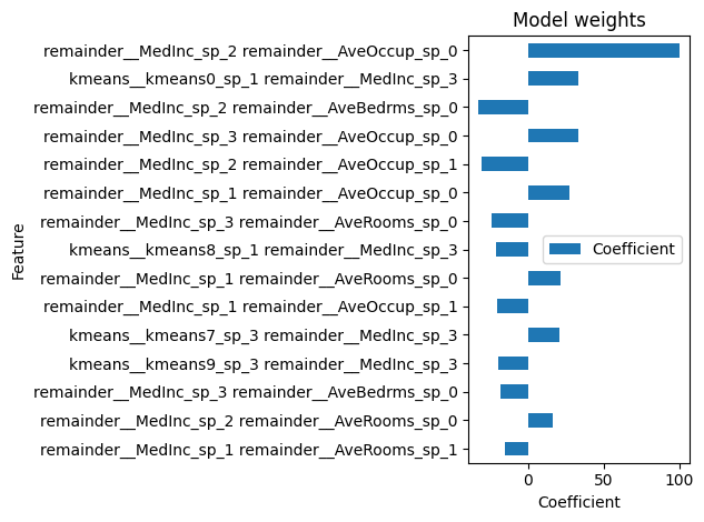
And here is the feature importance based on our model (sorted by absolute values):
(
    selectk_ridge_report.inspection.coefficients()
    .frame()
    .set_index("feature")
    .sort_values(by="coefficient", key=abs, ascending=True)
    .tail(15)
    .plot.barh(title="Model weights", xlabel="Coefficient", ylabel="Feature")
)
<Axes: title={'center': 'Model weights'}, xlabel='Coefficient', ylabel='Feature'>
Tree-based models: mean decrease in impurity (MDI)#
Now, let us look into tree-based models. For feature importance, we inspect their Mean Decrease in Impurity (MDI). The MDI of a feature is the normalized total reduction of the criterion (or loss) brought by that feature. The higher the MDI, the more important the feature.
Warning
The MDI is limited and can be misleading:
When features have large differences in cardinality, the MDI tends to favor those with higher cardinality. Fortunately, in this example, we have only numerical features that share similar cardinality, mitigating this concern.
Since the MDI is typically calculated on the training set, it can reflect biases from overfitting. When a model overfits, the tree may partition less relevant regions of the feature space, artificially inflating MDI values and distorting the perceived importance of certain features. Soon, scikit-learn will enable the computing of the MDI on the test set, and we will make it available in skore. Hence, we would be able to draw conclusions on how predictive a feature is and not just how impactful it is on the training procedure.
See also
For more information about the MDI, see scikit-learn’s Permutation Importance vs Random Forest Feature Importance (MDI).
Decision trees#
Let us start with a simple decision tree.
See also
For more information about decision trees, see scikit-learn’s example on Understanding the decision tree structure.
from sklearn.tree import DecisionTreeRegressor

tree_report = evaluate(DecisionTreeRegressor(random_state=0), X, y, splitter=0.2)
reports_to_compare["Decision tree"] = tree_report
We compare its performance with the models in our benchmark:
comparator = compare(reports_to_compare)
comparator.metrics.summarize().frame()
We note that the performance is quite poor, so the derived feature importance is to be dealt with caution.
We display which accessors are available to us:
We have a
impurity_decrease()
accessor.
First, let us interpret our model with regards to the original features.
For the visualization, we fix a very low max_depth so that it will be easy for
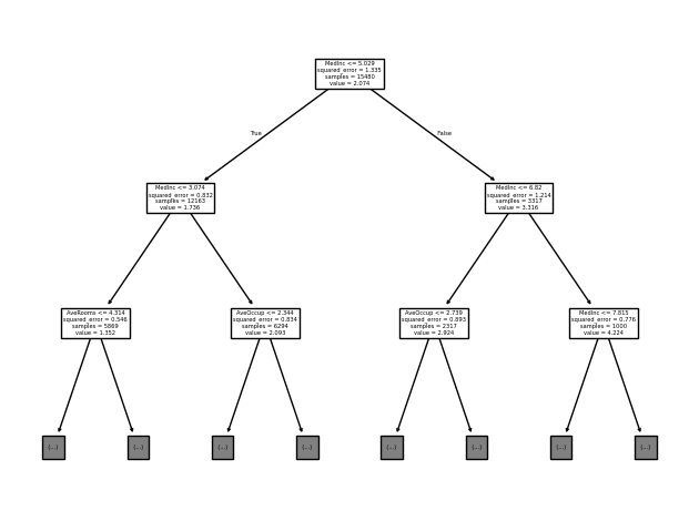
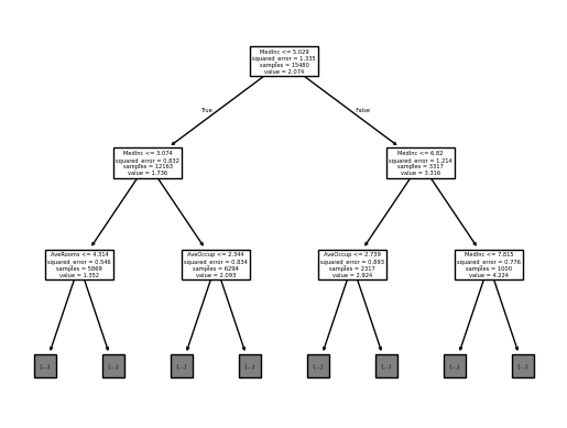
the human eye to visualize the tree using sklearn.tree.plot_tree():
from sklearn.tree import plot_tree

plot_tree(
    tree_report.estimator_,
    feature_names=tree_report.estimator_.feature_names_in_,
    max_depth=2,
)
[Text(0.5, 0.875, 'MedInc <= 5.029\nsquared_error = 1.338\nsamples = 16512\nvalue = 2.072'), Text(0.25, 0.625, 'MedInc <= 3.074\nsquared_error = 0.833\nsamples = 12979\nvalue = 1.733'), Text(0.375, 0.75, 'True '), Text(0.125, 0.375, 'AveRooms <= 4.314\nsquared_error = 0.545\nsamples = 6272\nvalue = 1.35'), Text(0.0625, 0.125, '\n (...) \n'), Text(0.1875, 0.125, '\n (...) \n'), Text(0.375, 0.375, 'AveOccup <= 2.373\nsquared_error = 0.836\nsamples = 6707\nvalue = 2.092'), Text(0.3125, 0.125, '\n (...) \n'), Text(0.4375, 0.125, '\n (...) \n'), Text(0.75, 0.625, 'MedInc <= 6.82\nsquared_error = 1.218\nsamples = 3533\nvalue = 3.319'), Text(0.625, 0.75, ' False'), Text(0.625, 0.375, 'AveOccup <= 2.74\nsquared_error = 0.891\nsamples = 2453\nvalue = 2.921'), Text(0.5625, 0.125, '\n (...) \n'), Text(0.6875, 0.125, '\n (...) \n'), Text(0.875, 0.375, 'MedInc <= 7.815\nsquared_error = 0.787\nsamples = 1080\nvalue = 4.222'), Text(0.8125, 0.125, '\n (...) \n'), Text(0.9375, 0.125, '\n (...) \n')]
This tree explains how each sample is going to be predicted by our tree. A decision tree provides a decision path for each sample, where the sample traverses the tree based on feature thresholds, and the final prediction is made at the leaf node (not represented above for conciseness purposes). At each node:
samplesis the number of samples that fall into that node,valueis the predicted output for the samples that fall into this particular node (it is the mean of the target values for the samples in that node). At the root node, the value is \(2.074\). This means that if you were to make a prediction for all \(15480\) samples at this node (without any further splits), the predicted value would be \(2.074\), which is the mean of the target variable for those samples.squared_erroris the mean squared error associated with thevalue, representing the average of the squared differences between the actual target values of the samples in the node and the node’s predictedvalue(the mean),the first element is how the split is defined.
Let us explain how this works in practice.
At each node, the tree splits the data based on a feature and a threshold.
For the first node (the root node), MedInc <= 5.029 means that, for each sample,
our decision tree first looks at the MedInc feature (which is thus the most
important one):
if the MedInc value is lower than \(5.029\) (the threshold), then the sample goes
into the left node, otherwise it goes to the right, and so on for each node.
As you move down the tree, the splits refine the predictions, leading to the leaf
nodes where the final prediction for a sample is the value of the leaf it reaches.
Note that for the second node layer, it is also the MedInc feature that is used
for the threshold, indicating that our model heavily relies on MedInc.
See also
A richer display of decision trees is available in the dtreeviz python package. For example, it shows the distribution of feature values split at each node and tailors the visualization to the task at hand (whether classification or regression).
Now, let us look at the feature importance based on the MDI:
_ = tree_report.inspection.impurity_decrease().plot()
For a decision tree, for each feature, the MDI is averaged across all splits in the tree. Here, the impurity is the mean squared error.
As expected, MedInc is of great importance for our decision tree.
Indeed, in the above tree visualization, MedInc is used multiple times for splits
and contributes greatly to reducing the squared error at multiple nodes.
At the root, it reduces the error from \(1.335\) to \(0.832\) and \(0.546\)
in the children.
Random forest#
Now, let us apply a more elaborate model: a random forest. A random forest is an ensemble method that builds multiple decision trees, each trained on a random subset of data and features. For regression, it averages the trees’ predictions. This reduces overfitting and improves accuracy compared to a single decision tree.
from sklearn.ensemble import RandomForestRegressor

n_estimators = 100
rf_report = evaluate(
    RandomForestRegressor(random_state=0, n_estimators=n_estimators), X, y, splitter=0.2
)
reports_to_compare["Random forest"] = rf_report

comparator = compare(reports_to_compare)
comparator.metrics.summarize().frame()
Without any feature engineering and any grid search, the random forest beats all linear models!
Let us recall the number of trees in our random forest:
print(f"Number of trees in the forest: {n_estimators}")
Number of trees in the forest: 100
Given that we have many trees, it is hard to use sklearn.tree.plot_tree() as
for the single decision tree.
As for linear models (and the complex feature engineering), better performance often
comes with less interpretability.
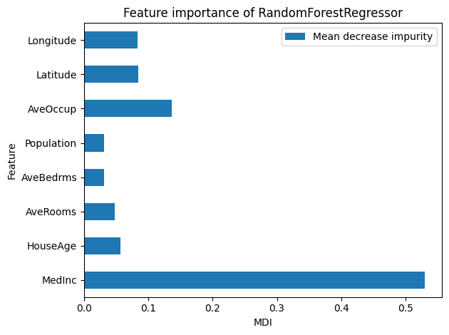
Let us look into the MDI of our random forest:
In a random forest, the MDI is computed by averaging the MDI of each feature across all the decision trees in the forest.
As for the decision tree, MecInc is the most important feature.
As for linear models with some feature engineering, the random forest also attributes
a high importance to Longitude, Latitude, and AveOccup.
Model-agnostic: permutation feature importance#
In the previous sections, we have inspected coefficients that are specific to linear models and the MDI that is specific to tree-based models. In this section, we look into the permutation importance which is model-agnostic, meaning that it can be applied to any fitted estimator. In particular, it works for linear models and tree-based ones.
Permutation feature importance measures the contribution of each feature to a fitted model’s performance. It randomly shuffles the values of a single feature and observes the resulting degradation of the model’s score. Permuting a predictive feature makes the performance decrease, while permuting a non-predictive feature does not degrade the performance much. This permutation importance can be computed on the train and test sets, and by default skore computes it on the test set. Compared to the coefficients and the MDI, the permutation importance can be less misleading, but comes with a higher computation cost.
Permutation feature importance can also help reduce overfitting. If a model overfits (high train score and low test score), and some features are important only on the train set and not on the test set, then these features might be the cause of the overfitting and it might be a good idea to drop them.
Warning
The permutation feature importance can be misleading on strongly correlated features. For more information, see scikit-learn’s user guide.
Now, let us look at our helper:
We have a permutation_importance()
accessor:
ridge_report.inspection.permutation_importance(seed=0).frame()
Since the permutation importance involves permuting values of a feature at random,
by default it is computed several times, each time with different permutations of
the feature. For this reason, if seed is not passed, skore does not cache the
permutation importance results.
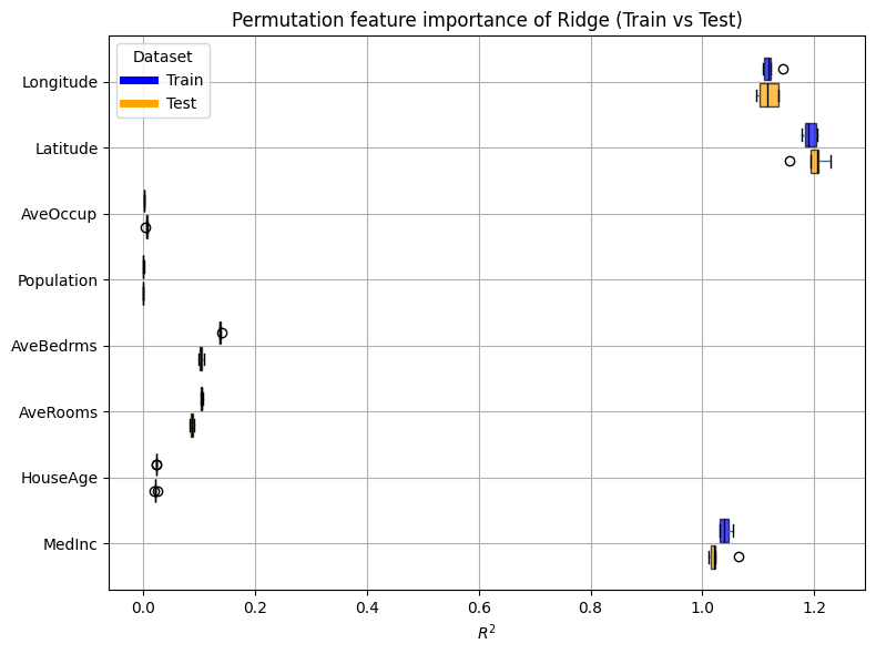
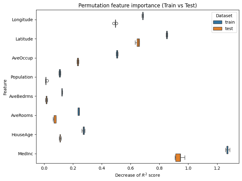
Now, we plot the permutation feature importance on the train and test sets using boxplots:
def plot_permutation_train_test(importances):
    _, ax = plt.subplots(figsize=(8, 6))

    sns.boxplot(
        data=importances,
        x="value",
        y="feature",
        hue="data_source",
        ax=ax,
        whis=10_000,
    )
    ax.set_xlabel("Decrease of $R^2$ score")
    ax.set_title("Permutation feature importance (Train vs Test)")
    plt.show(block=True)
def compute_permutation_importances(report, at_step=0):
    train_importance = report.inspection.permutation_importance(
        data_source="train", seed=0, at_step=at_step
    ).frame(aggregate=None)
    test_importance = report.inspection.permutation_importance(
        data_source="test", seed=0, at_step=at_step
    ).frame(aggregate=None)

    return pd.concat([train_importance, test_importance], axis=0)
plot_permutation_train_test(compute_permutation_importances(ridge_report))

The standard deviation seems quite low.
For both the train and test sets, the result of the inspection is the same as
with the coefficients:
the most important features are Latitude, Longitude, and MedInc.
For selectk_ridge_report, we have a large pipeline that is fed to a
EstimatorReport.
The pipeline contains a lot a preprocessing that creates many features.
By default, the permutation importance is calculated at the entrance of the whole
pipeline (with regards to the original features):
plot_permutation_train_test(compute_permutation_importances(selectk_ridge_report))
Since this estimator involves complex feature engineering, it is interesting to look at the impact of the engineered features rather than the original input features. For instance, we can check whether features with a low importance rating have indeed been selected out of the engineered features.
importances = compute_permutation_importances(selectk_ridge_report, at_step=-1)

# Rename some features for clarity
importances["feature"] = (
    importances["feature"]
    .str.replace("remainder__", "")
    .str.replace("kmeans__", "geospatial__")
)


# Take only the 15 most important train features
best_15_features = (
    importances.set_index("data_source")
    .loc["test", :]
    .drop(columns=["metric", "repetition"])
    .groupby("feature")
    .aggregate("mean")
    .sort_values(by="value", key=abs)
    .tail(15)
    .index
)
importances = importances.query("feature in @best_15_features")

plot_permutation_train_test(importances)

Hence, contrary to coefficients, although we have created many features in our preprocessing, the interpretability is easier. We notice that, due to our preprocessing using a clustering on the geospatial data, these features are of great importance to our model.
Also, Average Bedrooms and Average Rooms appear often in the plot, whereas they were not considered as important when looking at the coefficients. It means that once combined with other features, they become more relevant.
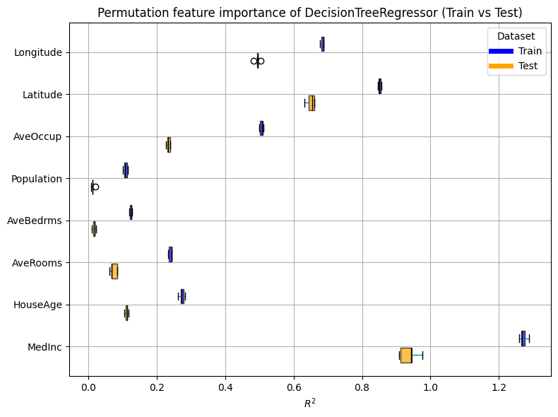
For our decision tree, here is our permutation importance on the train and test sets:
plot_permutation_train_test(compute_permutation_importances(tree_report))
The result of the inspection is the same as with the MDI:
the most important features are MedInc, Latitude, Longitude,
and AveOccup.
Conclusion#
In this example, we used the California housing dataset to predict house prices with
skore’s EstimatorReport.
By employing the inspection accessor,
we gained valuable insights into model behavior beyond mere predictive performance.
For linear models like Ridge regression, we inspected coefficients to understand
feature contributions, revealing the prominence of MedInc, Latitude,
and Longitude.
We explained the trade-off between performance (with complex feature engineering)
and interpretability.
Interactions between features have highlighted the importance of AveOccup.
With tree-based models such as decision trees, random forests, and gradient-boosted
trees, we utilized Mean Decrease in Impurity (MDI) to identify key features,
notably AveOccup alongside MedInc, Latitude, and
Longitude.
The random forest got the best score, without any complex feature engineering
compared to linear models.
The model-agnostic permutation feature importance further enabled us to compare
feature significance across diverse model types.
Total running time of the script: (1 minutes 32.450 seconds)