Note
Go to the end to download the full example code.
Skore: getting started#
This getting started guide illustrates how to use skore and why:
Get assistance when developing your machine learning projects to avoid common pitfalls and follow recommended practices.
skore.EstimatorReport: get an insightful report on your estimator, for evaluation and inspectionskore.CrossValidationReport: get an insightful report on your cross-validation resultsskore.ComparisonReport: benchmark your skore estimator reportsskore.train_test_split(): get diagnostics when splitting your data
Track your machine learning results using skore’s
Project(for storage).
Machine learning evaluation and diagnostics#
Skore implements new tools or wraps some key scikit-learn class / functions to automatically provide insights and diagnostics when using them, as a way to facilitate good practices and avoid common pitfalls.
Model evaluation with skore#
In order to assist its users when programming, skore has implemented a
skore.EstimatorReport class.
Let us create a challenging synthetic binary classification dataset and get the estimator report for a
RandomForestClassifier:
from sklearn.datasets import make_classification
from sklearn.ensemble import RandomForestClassifier
from sklearn.model_selection import train_test_split

from skore import EstimatorReport

X, y = make_classification(
    n_samples=10_000,
    n_classes=3,
    class_sep=0.3,
    n_clusters_per_class=1,
    random_state=42,
)
X_train, X_test, y_train, y_test = train_test_split(X, y, random_state=0)

rf = RandomForestClassifier(random_state=0)

rf_report = EstimatorReport(
    rf, X_train=X_train, X_test=X_test, y_train=y_train, y_test=y_test
)
Now, we can display the helper to see all the insights that are available to us (skore detected that we are doing multiclass classification):
╭───────────────── Tools to diagnose estimator RandomForestClassifier ─────────────────╮
│ EstimatorReport                                                                      │
│ ├── .metrics                                                                         │
│ │   ├── .accuracy(...)         (↗︎)     - Compute the accuracy score.                 │
│ │   ├── .confusion_matrix(...)         - Plot the confusion matrix.                  │
│ │   ├── .log_loss(...)         (↘︎)     - Compute the log loss.                       │
│ │   ├── .precision(...)        (↗︎)     - Compute the precision score.                │
│ │   ├── .precision_recall(...)         - Plot the precision-recall curve.            │
│ │   ├── .recall(...)           (↗︎)     - Compute the recall score.                   │
│ │   ├── .roc(...)                      - Plot the ROC curve.                         │
│ │   ├── .roc_auc(...)          (↗︎)     - Compute the ROC AUC score.                  │
│ │   ├── .timings(...)                  - Get all measured processing times related   │
│ │   │   to the estimator.                                                            │
│ │   ├── .custom_metric(...)            - Compute a custom metric.                    │
│ │   └── .summarize(...)                - Report a set of metrics for our estimator.  │
│ ├── .feature_importance                                                              │
│ │   ├── .mean_decrease_impurity(...)   - Retrieve the mean decrease impurity (MDI)   │
│ │   │   of a tree-based model.                                                       │
│ │   └── .permutation(...)              - Report the permutation feature importance.  │
│ ├── .data                                                                            │
│ │   └── .analyze(...)                  - Plot dataset statistics.                    │
│ ├── .cache_predictions(...)            - Cache estimator's predictions.              │
│ ├── .clear_cache(...)                  - Clear the cache.                            │
│ ├── .get_predictions(...)              - Get estimator's predictions.                │
│ └── Attributes                                                                       │
│     ├── .X_test                        - Testing data                                │
│     ├── .X_train                       - Training data                               │
│     ├── .y_test                        - Testing target                              │
│     ├── .y_train                       - Training target                             │
│     ├── .estimator                     - Estimator to make the report from           │
│     ├── .estimator_                    - The cloned or copied estimator              │
│     ├── .estimator_name_               - The name of the estimator                   │
│     ├── .fit                           - Whether to fit the estimator on the         │
│     │   training data                                                                │
│     ├── .fit_time_                     - The time taken to fit the estimator, in     │
│     │   seconds                                                                      │
│     ├── .ml_task                       - No description available                    │
│     └── .pos_label                     - For binary classification, the positive     │
│         class                                                                        │
│                                                                                      │
│                                                                                      │
│ Legend:                                                                              │
│ (↗︎) higher is better (↘︎) lower is better                                             │
╰──────────────────────────────────────────────────────────────────────────────────────╯
Note
This helper is great because:
it enables users to get a glimpse at the API of the different available accessors without having to look up the online documentation,
it provides methodological guidance: for example, we easily provide several metrics as a way to encourage users looking into them.
We can evaluate our model using the metrics() accessor.
In particular, we can get the report metrics that is computed for us (including the
fit and prediction times):
rf_report.metrics.summarize(indicator_favorability=True).frame()
For inspection, we can also retrieve the predictions, on the train set for example (here we display only the first 10 predictions for conciseness purposes):
rf_report.get_predictions(data_source="train")[0:10]
array([2, 1, 2, 2, 2, 1, 0, 0, 0, 0])
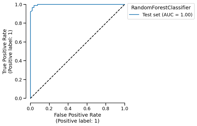
We can also plot the ROC curve that is generated for us:
roc_plot = rf_report.metrics.roc()
roc_plot.plot()
Furthermore, we can inspect our model using the
feature_importance() accessor.
In particular, we can inspect the model using the permutation feature importance:
rf_report.feature_importance.permutation(seed=0).T.boxplot(vert=False)
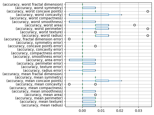
<Axes: >
See also
For more information about the motivation and usage of
skore.EstimatorReport, see the following use cases:
EstimatorReport: Get insights from any scikit-learn estimator for model evaluation,
EstimatorReport: Inspecting your models with the feature importance for model inspection.
Cross-validation with skore#
skore has also (re-)implemented a skore.CrossValidationReport class that
contains several skore.EstimatorReport, one for each split.
from skore import CrossValidationReport

cv_report = CrossValidationReport(rf, X, y, splitter=5)
We display the cross-validation report helper:
╭───────────────── Tools to diagnose estimator RandomForestClassifier ─────────────────╮
│ CrossValidationReport                                                                │
│ ├── .metrics                                                                         │
│ │   ├── .accuracy(...)         (↗︎)     - Compute the accuracy score.                 │
│ │   ├── .log_loss(...)         (↘︎)     - Compute the log loss.                       │
│ │   ├── .precision(...)        (↗︎)     - Compute the precision score.                │
│ │   ├── .precision_recall(...)         - Plot the precision-recall curve.            │
│ │   ├── .recall(...)           (↗︎)     - Compute the recall score.                   │
│ │   ├── .roc(...)                      - Plot the ROC curve.                         │
│ │   ├── .roc_auc(...)          (↗︎)     - Compute the ROC AUC score.                  │
│ │   ├── .timings(...)                  - Get all measured processing times related   │
│ │   │   to the estimator.                                                            │
│ │   ├── .custom_metric(...)            - Compute a custom metric.                    │
│ │   └── .summarize(...)                - Report a set of metrics for our estimator.  │
│ ├── .feature_importance                                                              │
│ ├── .cache_predictions(...)            - Cache the predictions for sub-estimators    │
│ │   reports.                                                                         │
│ ├── .clear_cache(...)                  - Clear the cache.                            │
│ ├── .get_predictions(...)              - Get estimator's predictions.                │
│ └── Attributes                                                                       │
│     ├── .X                             - The data to fit                             │
│     ├── .y                             - The target variable to try to predict in    │
│     │   the case of supervised learning                                              │
│     ├── .estimator                     - Estimator to make the cross-validation      │
│     │   report from                                                                  │
│     ├── .estimator_                    - The cloned or copied estimator              │
│     ├── .estimator_name_               - The name of the estimator                   │
│     ├── .estimator_reports_            - The estimator reports for each split        │
│     ├── .ml_task                       - No description available                    │
│     ├── .n_jobs                        - Number of jobs to run in parallel           │
│     ├── .pos_label                     - For binary classification, the positive     │
│     │   class                                                                        │
│     ├── .split_indices                 - No description available                    │
│     └── .splitter                      - Determines the cross-validation splitting   │
│         strategy                                                                     │
│                                                                                      │
│                                                                                      │
│ Legend:                                                                              │
│ (↗︎) higher is better (↘︎) lower is better                                             │
╰──────────────────────────────────────────────────────────────────────────────────────╯
We display the mean and standard deviation for each metric:
cv_report.metrics.summarize().frame()
or by individual split:
cv_report.metrics.summarize(aggregate=None).frame()
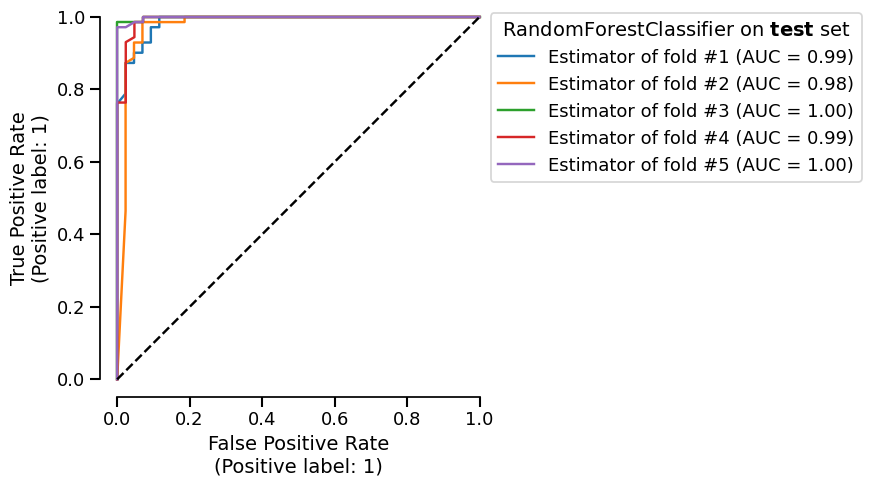
We display the ROC curves for each split:
roc_plot_cv = cv_report.metrics.roc()
roc_plot_cv.plot()
We can retrieve the estimator report of a specific split to investigate further, for example getting the report metrics for the first split only:
cv_report.estimator_reports_[0].metrics.summarize().frame()
See also
For more information about the motivation and usage of
skore.CrossValidationReport, see Simplified and structured experiment reporting.
Comparing estimator reports#
skore.ComparisonReport enables users to compare several estimator reports
(corresponding to several estimators) on a same test set, as in a benchmark of
estimators.
Apart from the previous rf_report, let us define another estimator report:
from sklearn.ensemble import GradientBoostingClassifier

gb = GradientBoostingClassifier(random_state=0)
gb_report = EstimatorReport(
    gb, X_train=X_train, X_test=X_test, y_train=y_train, y_test=y_test, pos_label=1
)
We can conveniently compare our two estimator reports, that were applied to the exact same test set:
from skore import ComparisonReport

comparator = ComparisonReport(reports=[rf_report, gb_report])
As for the EstimatorReport and the
CrossValidationReport, we have a helper:
╭──────────────────────────── Tools to compare estimators ─────────────────────────────╮
│ ComparisonReport                                                                     │
│ ├── .metrics                                                                         │
│ │   ├── .accuracy(...)         (↗︎)     - Compute the accuracy score.                 │
│ │   ├── .log_loss(...)         (↘︎)     - Compute the log loss.                       │
│ │   ├── .precision(...)        (↗︎)     - Compute the precision score.                │
│ │   ├── .precision_recall(...)         - Plot the precision-recall curve.            │
│ │   ├── .recall(...)           (↗︎)     - Compute the recall score.                   │
│ │   ├── .roc(...)                      - Plot the ROC curve.                         │
│ │   ├── .roc_auc(...)          (↗︎)     - Compute the ROC AUC score.                  │
│ │   ├── .timings(...)                  - Get all measured processing times related   │
│ │   │   to the different estimators.                                                 │
│ │   ├── .custom_metric(...)            - Compute a custom metric.                    │
│ │   └── .summarize(...)                - Report a set of metrics for the estimators. │
│ ├── .feature_importance                                                              │
│ ├── .cache_predictions(...)            - Cache the predictions for sub-estimators    │
│ │   reports.                                                                         │
│ ├── .clear_cache(...)                  - Clear the cache.                            │
│ ├── .get_predictions(...)              - Get predictions from the underlying         │
│ │   reports.                                                                         │
│ └── Attributes                                                                       │
│     ├── .n_jobs                        - Number of jobs to run in parallel           │
│     ├── .pos_label                     - No description available                    │
│     └── .reports_                      - The compared reports                        │
│                                                                                      │
│                                                                                      │
│ Legend:                                                                              │
│ (↗︎) higher is better (↘︎) lower is better                                             │
╰──────────────────────────────────────────────────────────────────────────────────────╯
Let us display the result of our benchmark:
comparator.metrics.summarize(indicator_favorability=True).frame()
Thus, we easily have the result of our benchmark for several recommended metrics.
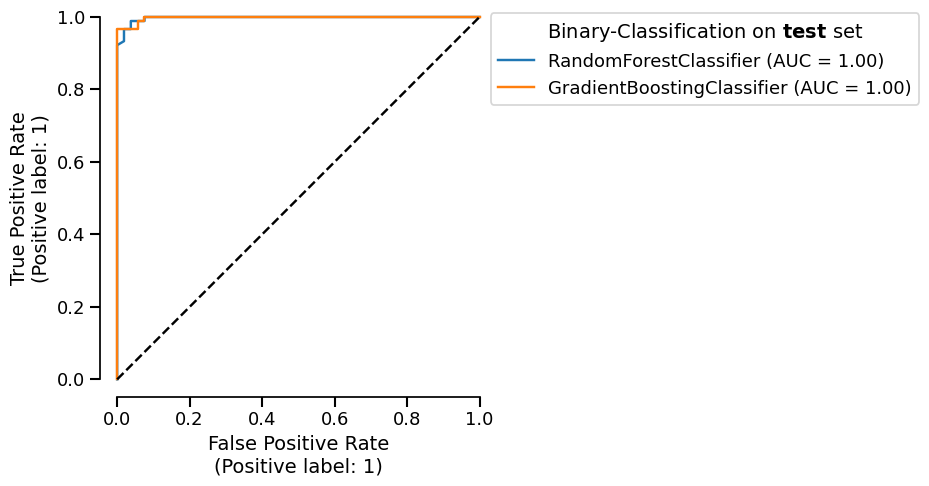
Moreover, we can display the ROC curve for the two estimator reports we want to compare, by superimposing them on the same figure:
comparator.metrics.roc().plot()
Train-test split with skore#
Skore has implemented a skore.train_test_split() function that wraps
scikit-learn’s sklearn.model_selection.train_test_split().
Let us load a dataset containing some time series data:
import pandas as pd
from skrub.datasets import fetch_employee_salaries

dataset_employee = fetch_employee_salaries()
X_employee, y_employee = dataset_employee.X, dataset_employee.y
X_employee["date_first_hired"] = pd.to_datetime(
    X_employee["date_first_hired"], format="%m/%d/%Y"
)
X_employee.head(2)
Downloading 'employee_salaries' from https://github.com/skrub-data/skrub-data-files/raw/refs/heads/main/employee_salaries.zip (attempt 1/3)
We can observe that there is a date_first_hired which is time-based.
Now, let us apply skore.train_test_split() on this data:
import skore

_ = skore.train_test_split(
    X=X_employee, y=y_employee, random_state=0, shuffle=False, as_dict=True
)
╭─────────────────────────────── TimeBasedColumnWarning ───────────────────────────────╮
│ We detected some time-based columns (column "date_first_hired") in your data. We     │
│ recommend using scikit-learn's TimeSeriesSplit instead of train_test_split.          │
│ Otherwise you might train on future data to predict the past, or get inflated model  │
│ performance evaluation because natural drift will not be taken into account.         │
╰──────────────────────────────────────────────────────────────────────────────────────╯
We get a TimeBasedColumnWarning advising us to use
sklearn.model_selection.TimeSeriesSplit instead!
Indeed, we should not shuffle time-ordered data!
See also
More methodological advice is available.
For more information about the motivation and usage of
skore.train_test_split(), see train_test_split: get diagnostics when splitting your data.
Tracking: skore project#
Another key feature of skore is its Project that allows us to store
and retrieve EstimatorReport objects.
Setup: creating and loading a skore project#
Let us start by creating a skore project named my_project:
my_project = skore.Project("my_project")
Storing some reports in our project#
Now that the project exists, we can store some useful reports in it using
put(), with a key-value convention.
Let us store the estimator reports of the random forest and the gradient boosting to help us track our experiments:
my_project.put("estimator_report", rf_report)
my_project.put("estimator_report", gb_report)
Retrieving our stored reports#
Now, let us retrieve the data that we just stored using a
Summary object:
summary = my_project.summarize()
print(type(summary))
<class 'skore.project.summary.Summary'>
We can retrieve the complete list of stored reports:
from pprint import pprint

reports_get = summary.reports()
pprint(reports_get)
[EstimatorReport(estimator=RandomForestClassifier(random_state=0), ...),
 EstimatorReport(estimator=GradientBoostingClassifier(random_state=0), ...)]
For example, we can compare the stored reports:
comparator = ComparisonReport(reports=reports_get)
comparator.metrics.summarize(pos_label=1, indicator_favorability=True).frame()
We can retrieve any accessor of our stored estimator reports, for example the timings from the first estimator report:
reports_get[0].metrics.timings()
{'fit_time': 3.476288230000023, 'predict_time_test': 0.03270254300002762}
But what if instead of having stored only 2 estimators reports, we had a dozen or even a few hundreds over several months of experimenting? We would need to navigate through our stored estimator reports. For that, the skore project provides a convenient search feature.
Searching through our stored reports#
Using the interactive widget#
If rendered in a Jupyter notebook, summary would render an interactive
parallel coordinate plot to search for your preferred model based on some metrics.
Here is a screenshot:
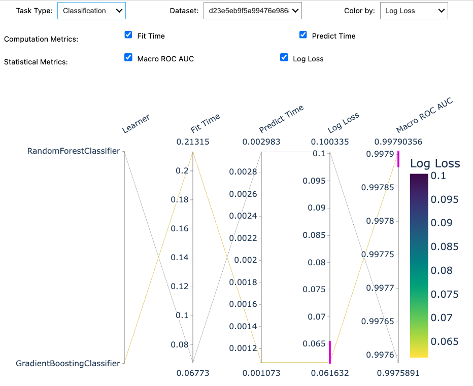
How to use the widget? You select the estimator(s) you are interested in by clicking on the plot and the metric(s) you are interested in by checking them. Then, using the python API, we can retrieve the corresponding list of stored reports:
Using the Python API#
Alternatively, this search feature can be performed using the Python API.
We can perform some queries on our stored data using the following keys:
Index(['key', 'date', 'learner', 'ml_task', 'report_type', 'dataset', 'rmse',
       'log_loss', 'roc_auc', 'fit_time', 'predict_time', 'rmse_mean',
       'log_loss_mean', 'roc_auc_mean', 'fit_time_mean', 'predict_time_mean'],
      dtype='object')
For example, we can query all the estimators corresponding to a
RandomForestClassifier:
report_search_rf = summary.query(
    "learner.str.contains('RandomForestClassifier')"
).reports()
pprint(report_search_rf)
[EstimatorReport(estimator=RandomForestClassifier(random_state=0), ...)]
Or, we can query all the estimator reports corresponding to a classification task:
report_search_clf = summary.query("ml_task.str.contains('classification')").reports()
pprint(report_search_clf)
[EstimatorReport(estimator=RandomForestClassifier(random_state=0), ...),
 EstimatorReport(estimator=GradientBoostingClassifier(random_state=0), ...)]
Stay tuned!
These are only the initial features: skore is a work in progress and aims to be an end-to-end library for data scientists.
Feedbacks are welcome: please feel free to join our Discord or create an issue.
Total running time of the script: (0 minutes 46.423 seconds)