Simplified and structured experiment reporting

This example shows how to leverage skore for structuring useful experiment information allowing to get insights from machine learning experiments.

We set some environment variables to avoid some spurious warnings related to parallelism when using the TextEncoder from skrub that uses tokenizers.

import os

os.environ["TOKENIZERS_PARALLELISM"] = "true"

Loading a non-trivial dataset

We use a skrub dataset that contains information about employees and their salaries. We will see that this dataset is non-trivial.

from skrub.datasets import fetch_employee_salaries

datasets = fetch_employee_salaries()
df, y = datasets.X, datasets.y

Let’s first have a condensed summary of the input data using a skrub.TableReport.

from skrub import TableReport

TableReport(df)

Please enable javascript

The skrub table reports need javascript to display correctly. If you are displaying a report in a Jupyter notebook and you see this message, you may need to re-execute the cell or to trust the notebook (button on the top right or "File > Trust notebook").

From the table report, we can make the following observations:

• Looking at the Table tab, we observe that the year related to the date_first_hired column is also present in the date column. Hence, we should beware of not creating twice the same feature during the feature engineering.

• Looking at the Stats tab:

  • The type of data is heterogeneous: we mainly have categorical and date-related features.

  • The division and employee_position_title features contain a large number of categories. It is something that we should consider in our feature engineering.

• Looking at the Associations tab, we observe that two features are holding the exact same information: department and department_name. Hence, during our feature engineering, we could potentially drop one of them if the final predictive model is sensitive to the collinearity.

In terms of target and thus the task that we want to solve, we are interested in predicting the salary of an employee given the previous features. We therefore have a regression task at end.

TableReport(y)

Please enable javascript

The skrub table reports need javascript to display correctly. If you are displaying a report in a Jupyter notebook and you see this message, you may need to re-execute the cell or to trust the notebook (button on the top right or "File > Trust notebook").

Later in this example, we will show that skore stores similar information when a model is trained on a dataset, thus enabling us to get quick insights on the dataset used to train and test the model.

Tree-based model

Let’s start by creating a tree-based model using some out-of-the-box tools.

For feature engineering, we use skrub’s TableVectorizer. To deal with the high cardinality of the categorical features, we use a TextEncoder that uses a language model and an embedding model to encode the categorical features.

Finally, we use a HistGradientBoostingRegressor as a base estimator, it is a rather robust model.

Modelling

from skrub import TableVectorizer, TextEncoder
from sklearn.ensemble import HistGradientBoostingRegressor
from sklearn.pipeline import make_pipeline

model = make_pipeline(
    TableVectorizer(high_cardinality=TextEncoder()),
    HistGradientBoostingRegressor(),
)
model

Pipeline(steps=[('tablevectorizer',
                 TableVectorizer(high_cardinality=TextEncoder())),
                ('histgradientboostingregressor',
                 HistGradientBoostingRegressor())])

In a Jupyter environment, please rerun this cell to show the HTML representation or trust the notebook.
On GitHub, the HTML representation is unable to render, please try loading this page with nbviewer.org.

Evaluation

Let us compute the cross-validation report for this model using a skore.CrossValidationReport:

from skore import CrossValidationReport

hgbt_model_report = CrossValidationReport(
    estimator=model, X=df, y=y, splitter=5, n_jobs=4
)
hgbt_model_report.help()

╭───────────── Tools to diagnose estimator HistGradientBoostingRegressor ──────────────╮
│ CrossValidationReport                                                                │
│ ├── .metrics                                                                         │
│ │   ├── .prediction_error(...)         - Plot the prediction error of a regression   │
│ │   │   model.                                                                       │
│ │   ├── .r2(...)               (↗︎)     - Compute the R² score.                       │
│ │   ├── .rmse(...)             (↘︎)     - Compute the root mean squared error.        │
│ │   ├── .timings(...)                  - Get all measured processing times related   │
│ │   │   to the estimator.                                                            │
│ │   ├── .custom_metric(...)            - Compute a custom metric.                    │
│ │   └── .summarize(...)                - Report a set of metrics for our estimator.  │
│ ├── .cache_predictions(...)            - Cache the predictions for sub-estimators    │
│ │   reports.                                                                         │
│ ├── .clear_cache(...)                  - Clear the cache.                            │
│ ├── .get_predictions(...)              - Get estimator's predictions.                │
│ └── Attributes                                                                       │
│     ├── .X                             - The data to fit                             │
│     ├── .y                             - The target variable to try to predict in    │
│     │   the case of supervised learning                                              │
│     ├── .estimator                     - Estimator to make the cross-validation      │
│     │   report from                                                                  │
│     ├── .estimator_                    - The cloned or copied estimator              │
│     ├── .estimator_name_               - The name of the estimator                   │
│     ├── .estimator_reports_            - The estimator reports for each split        │
│     ├── .ml_task                       - No description available                    │
│     ├── .n_jobs                        - Number of jobs to run in parallel           │
│     ├── .pos_label                     - For binary classification, the positive     │
│     │   class                                                                        │
│     ├── .split_indices                 - No description available                    │
│     └── .splitter                      - Determines the cross-validation splitting   │
│         strategy                                                                     │
│                                                                                      │
│                                                                                      │
│ Legend:                                                                              │
│ (↗︎) higher is better (↘︎) lower is better                                             │
╰──────────────────────────────────────────────────────────────────────────────────────╯

A report provides a collection of useful information. For instance, it allows to compute on demand the predictions of the model and some performance metrics.

Let’s cache the predictions of the cross-validated models once and for all.

hgbt_model_report.cache_predictions(n_jobs=4)

Now that the predictions are cached, any request to compute a metric will be performed using the cached predictions and will thus be fast.

We can now have a look at the performance of the model with some standard metrics.

hgbt_model_report.metrics.summarize().frame()

	HistGradientBoostingRegressor
	mean	std
Metric
R²	0.924282	0.017469
RMSE	7991.516753	1195.815810
Fit time (s)	17.865792	5.315400
Predict time (s)	14.827678	20.325525

Similarly to what we saw in the previous section, the skore.CrossValidationReport also stores some information about the dataset used.

data_display = hgbt_model_report.data.analyze()
data_display

Please enable javascript

The skrub table reports need javascript to display correctly. If you are displaying a report in a Jupyter notebook and you see this message, you may need to re-execute the cell or to trust the notebook (button on the top right or "File > Trust notebook").

The display obtained allows for a quick overview with the same HTML-based view as the skrub.TableReport we have seen earlier. In addition, you can access a skore.TableReportDisplay.plot() method to have a particular focus on one potential analysis. For instance, we can get a figure representing the correlation matrix of the dataset.

data_display.plot(kind="corr")

We get the results from some statistical metrics aggregated over the cross-validation splits as well as some performance metrics related to the time it took to train and test the model.

The skore.CrossValidationReport also provides a way to inspect similar information at the level of each cross-validation split by accessing an skore.EstimatorReport for each split.

hgbt_split_1 = hgbt_model_report.estimator_reports_[0]
hgbt_split_1.metrics.summarize(indicator_favorability=True).frame()

	HistGradientBoostingRegressor	Favorability
Metric
R²	0.922033	(↗︎)
RMSE	8040.374042	(↘︎)
Fit time (s)	20.083199	(↘︎)
Predict time (s)	5.063689	(↘︎)

The favorability of each metric indicates whether the metric is better when higher or lower.

Linear model

Now that we have established a first model that serves as a baseline, we shall proceed to define a quite complex linear model: a pipeline with a complex feature engineering that uses a linear model as the base estimator.

Modelling

import numpy as np
from sklearn.compose import make_column_transformer
from sklearn.pipeline import make_pipeline
from sklearn.preprocessing import OneHotEncoder, SplineTransformer
from sklearn.linear_model import RidgeCV
from skrub import DatetimeEncoder, ToDatetime, DropCols, GapEncoder


def periodic_spline_transformer(period, n_splines=None, degree=3):
    if n_splines is None:
        n_splines = period
    n_knots = n_splines + 1  # periodic and include_bias is True
    return SplineTransformer(
        degree=degree,
        n_knots=n_knots,
        knots=np.linspace(0, period, n_knots).reshape(n_knots, 1),
        extrapolation="periodic",
        include_bias=True,
    )


one_hot_features = ["gender", "department_name", "assignment_category"]
datetime_features = "date_first_hired"

date_encoder = make_pipeline(
    ToDatetime(),
    DatetimeEncoder(resolution="day", add_weekday=True, add_total_seconds=False),
    DropCols("date_first_hired_year"),
)

date_engineering = make_column_transformer(
    (periodic_spline_transformer(12, n_splines=6), ["date_first_hired_month"]),
    (periodic_spline_transformer(31, n_splines=15), ["date_first_hired_day"]),
    (periodic_spline_transformer(7, n_splines=3), ["date_first_hired_weekday"]),
)

feature_engineering_date = make_pipeline(date_encoder, date_engineering)

preprocessing = make_column_transformer(
    (feature_engineering_date, datetime_features),
    (OneHotEncoder(drop="if_binary", handle_unknown="ignore"), one_hot_features),
    (GapEncoder(n_components=100), "division"),
    (GapEncoder(n_components=100), "employee_position_title"),
)

model = make_pipeline(preprocessing, RidgeCV(alphas=np.logspace(-3, 3, 100)))
model

Pipeline(steps=[('columntransformer',
                 ColumnTransformer(transformers=[('pipeline',
                                                  Pipeline(steps=[('pipeline',
                                                                   Pipeline(steps=[('todatetime',
                                                                                    ToDatetime()),
                                                                                   ('datetimeencoder',
                                                                                    DatetimeEncoder(add_total_seconds=False,
                                                                                                    add_weekday=True,
                                                                                                    resolution='day')),
                                                                                   ('dropcols',
                                                                                    DropCols(cols='date_first_hired_year'))])),
                                                                  ('columntransformer',
                                                                   ColumnTransformer(transfor...
       4.03701726e+01, 4.64158883e+01, 5.33669923e+01, 6.13590727e+01,
       7.05480231e+01, 8.11130831e+01, 9.32603347e+01, 1.07226722e+02,
       1.23284674e+02, 1.41747416e+02, 1.62975083e+02, 1.87381742e+02,
       2.15443469e+02, 2.47707636e+02, 2.84803587e+02, 3.27454916e+02,
       3.76493581e+02, 4.32876128e+02, 4.97702356e+02, 5.72236766e+02,
       6.57933225e+02, 7.56463328e+02, 8.69749003e+02, 1.00000000e+03])))])

In a Jupyter environment, please rerun this cell to show the HTML representation or trust the notebook.
On GitHub, the HTML representation is unable to render, please try loading this page with nbviewer.org.

In the diagram above, we can see what how we performed our feature engineering:

• For categorical features, we use two approaches. If the number of categories is relatively small, we use a OneHotEncoder. If the number of categories is large, we use a GapEncoder that is designed to deal with high cardinality categorical features.

• Then, we have another transformation to encode the date features. We first split the date into multiple features (day, month, and year). Then, we apply a periodic spline transformation to each of the date features in order to capture the periodicity of the data.

• Finally, we fit a RidgeCV model.

Evaluation

Now, we want to evaluate this linear model via cross-validation (with 5 folds). For that, we use skore’s CrossValidationReport to investigate the performance of our model.

linear_model_report = CrossValidationReport(
    estimator=model, X=df, y=y, splitter=5, n_jobs=4
)
linear_model_report.help()

╭──────────────────────── Tools to diagnose estimator RidgeCV ─────────────────────────╮
│ CrossValidationReport                                                                │
│ ├── .metrics                                                                         │
│ │   ├── .prediction_error(...)         - Plot the prediction error of a regression   │
│ │   │   model.                                                                       │
│ │   ├── .r2(...)               (↗︎)     - Compute the R² score.                       │
│ │   ├── .rmse(...)             (↘︎)     - Compute the root mean squared error.        │
│ │   ├── .timings(...)                  - Get all measured processing times related   │
│ │   │   to the estimator.                                                            │
│ │   ├── .custom_metric(...)            - Compute a custom metric.                    │
│ │   └── .summarize(...)                - Report a set of metrics for our estimator.  │
│ ├── .cache_predictions(...)            - Cache the predictions for sub-estimators    │
│ │   reports.                                                                         │
│ ├── .clear_cache(...)                  - Clear the cache.                            │
│ ├── .get_predictions(...)              - Get estimator's predictions.                │
│ └── Attributes                                                                       │
│     ├── .X                             - The data to fit                             │
│     ├── .y                             - The target variable to try to predict in    │
│     │   the case of supervised learning                                              │
│     ├── .estimator                     - Estimator to make the cross-validation      │
│     │   report from                                                                  │
│     ├── .estimator_                    - The cloned or copied estimator              │
│     ├── .estimator_name_               - The name of the estimator                   │
│     ├── .estimator_reports_            - The estimator reports for each split        │
│     ├── .ml_task                       - No description available                    │
│     ├── .n_jobs                        - Number of jobs to run in parallel           │
│     ├── .pos_label                     - For binary classification, the positive     │
│     │   class                                                                        │
│     ├── .split_indices                 - No description available                    │
│     └── .splitter                      - Determines the cross-validation splitting   │
│         strategy                                                                     │
│                                                                                      │
│                                                                                      │
│ Legend:                                                                              │
│ (↗︎) higher is better (↘︎) lower is better                                             │
╰──────────────────────────────────────────────────────────────────────────────────────╯

We observe that the cross-validation report has detected that we have a regression task at hand and thus provides us with some metrics and plots that make sense with regards to our specific problem at hand.

To accelerate any future computation (e.g. of a metric), we cache the predictions of our model once and for all. Note that we do not necessarily need to cache the predictions as the report will compute them on the fly (if not cached) and cache them for us.

import warnings

with warnings.catch_warnings():
    warnings.simplefilter(action="ignore", category=FutureWarning)
    linear_model_report.cache_predictions(n_jobs=4)

We can now have a look at the performance of the model with some standard metrics.

linear_model_report.metrics.summarize(indicator_favorability=True).frame()

	RidgeCV		Favorability
	mean	std
Metric
R²	0.763934	0.023739	(↗︎)
RMSE	14142.005429	1217.774191	(↘︎)
Fit time (s)	11.110421	2.575626	(↘︎)
Predict time (s)	0.408760	0.004272	(↘︎)

Comparing the models

Now that we cross-validated our models, we can make some further comparison using the skore.ComparisonReport:

from skore import ComparisonReport

comparator = ComparisonReport([hgbt_model_report, linear_model_report])
comparator.metrics.summarize(indicator_favorability=True).frame()

	mean		std		Favorability
Estimator	HistGradientBoostingRegressor	RidgeCV	HistGradientBoostingRegressor	RidgeCV
Metric
R²	0.924282	0.763934	0.017469	0.023739	(↗︎)
RMSE	7991.516753	14142.005429	1195.815810	1217.774191	(↘︎)
Fit time (s)	17.865792	11.110421	5.315400	2.575626	(↘︎)
Predict time (s)	14.827678	0.408760	20.325525	0.004272	(↘︎)

In addition, if we forgot to compute a specific metric (e.g. mean_absolute_error()), we can easily add it to the report, without re-training the model and even without re-computing the predictions since they are cached internally in the report. This allows us to save some potentially huge computation time.

from sklearn.metrics import get_scorer

scoring = ["r2", "rmse", get_scorer("neg_mean_absolute_error")]
scoring_kwargs = {"response_method": "predict"}
scoring_names = ["R²", "RMSE", "MAE"]

comparator.metrics.summarize(
    scoring=scoring,
    scoring_kwargs=scoring_kwargs,
    scoring_names=scoring_names,
).frame()

	mean		std
Estimator	HistGradientBoostingRegressor	RidgeCV	HistGradientBoostingRegressor	RidgeCV
Metric
R²	0.924282	0.763934	0.017469	0.023739
RMSE	7991.516753	14142.005429	1195.815810	1217.774191
MAE	4433.515526	9886.685773	251.650830	551.519807

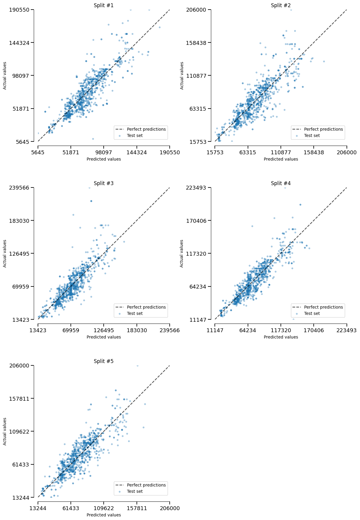
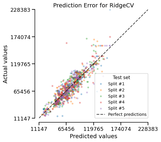
Finally, we can even get a deeper understanding by analyzing each split in the CrossValidationReport. Here, we plot the actual-vs-predicted values for each split.

linear_model_report.metrics.prediction_error().plot(kind="actual_vs_predicted")

Conclusion

This example showcased skore’s integrated approach to machine learning workflow, from initial data exploration with TableReport through model development and evaluation with CrossValidationReport. We demonstrated how skore automatically captures dataset information and provides efficient caching, enabling quick insights and flexible model comparison. The workflow highlights skore’s ability to streamline the entire ML process while maintaining computational efficiency.