Using skore with scikit-learn compatible estimators

This example shows how to use skore with scikit-learn compatible estimators.

Any model that can be used with the scikit-learn API can be used with skore. Use evaluate() to create a report from any estimator that has a fit and predict method (or only predict if already fitted).

Note

When computing the ROC AUC or ROC curve for a classification task, the estimator must have a predict_proba method.

In this example, we showcase a gradient boosting model (XGBoost) and a custom estimator.

Note that this example is not exhaustive; many other scikit-learn compatible models can be used with skore:

• More gradient boosting libraries like LightGBM, and CatBoost,

• Deep learning frameworks such as Keras and skorch (a wrapper for PyTorch).

• Tabular foundation models such as TabICL and TabPFN,

• etc.

Generate a classification dataset

To illustrate the compatibility with scikit-learn estimators, we first generate a synthetic binary classification dataset with only 1,000 samples.

import pandas as pd
import skrub
from sklearn.datasets import make_classification

X, y = make_classification(n_samples=1_000, random_state=42)
X = pd.DataFrame(X, columns=[f"Feature_{i}" for i in range(X.shape[1])])
skrub.TableReport(X)

Please enable javascript

The skrub table reports need javascript to display correctly. If you are displaying a report in a Jupyter notebook and you see this message, you may need to re-execute the cell or to trust the notebook (button on the top right or "File > Trust notebook").

Gradient-boosted decision trees with XGBoost

While skore is designed to be fully compatible with classifiers and regressors from the scikit-learn library, it is also compatible with any classifier or regressor that follows the scikit-learn API as defined in the scikit-learn documentation.

Here, we showcase a gradient-boosted decision trees model from the XGBoost library that follows exactly this paradigm.

from skore import evaluate
from xgboost import XGBClassifier

xgb = XGBClassifier(n_estimators=50, max_depth=3, learning_rate=0.1, random_state=42)

xgb_report = evaluate(xgb, X, y, splitter=0.2, pos_label=1)
xgb_report

XGBClassifier(base_score=None, booster=None, callbacks=None,
              colsample_bylevel=None, colsample_bynode=None,
              colsample_bytree=None, device=None, early_stopping_rounds=None,
              enable_categorical=False, eval_metric=None, feature_types=None,
              feature_weights=None, gamma=None, grow_policy=None,
              importance_type=None, interaction_constraints=None,
              learning_rate=0.1, max_bin=None, max_cat_threshold=None,
              max_cat_to_onehot=None, max_delta_step=None, max_depth=3,
              max_leaves=None, min_child_weight=None, missing=nan,
              monotone_constraints=None, multi_strategy=None, n_estimators=50,
              n_jobs=None, num_parallel_tree=None, ...)

In a Jupyter environment, please rerun this cell to show the HTML representation or trust the notebook.
On GitHub, the HTML representation is unable to render, please try loading this page with nbviewer.org.

Please enable javascript

The skrub table reports need javascript to display correctly. If you are displaying a report in a Jupyter notebook and you see this message, you may need to re-execute the cell or to trust the notebook (button on the top right or "File > Trust notebook").

0 issue(s), 0 tip(s), 3 passed, 0 ignored.

We see that we get the same report as when using a scikit-learn classifier and we can access the different elements.

xgb_report.metrics.summarize().frame()

	XGBClassifier
Metric
Accuracy	0.900000
Precision	0.989899
Recall	0.837607
ROC AUC	0.980126
Log loss	0.218888
Brier score	0.064364
Fit time (s)	0.039216
Predict time (s)	0.001271

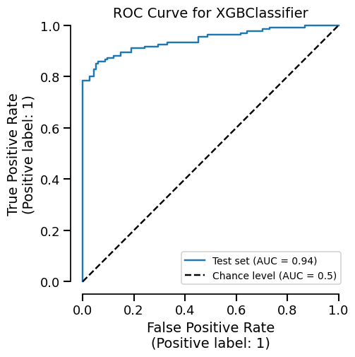
We can easily get the summary of metrics, and also a ROC curve plot for example:

_ = xgb_report.metrics.roc().plot()

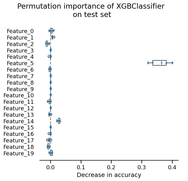
We can also inspect our model:

_ = xgb_report.inspection.permutation_importance().plot()

Custom model

Now, we showcase how one could create a scikit-learn custom estimator that follows the requirements of scikit-learn.

Here, we create a nearest neighbor classifier:

import numpy as np
from sklearn.base import BaseEstimator, ClassifierMixin
from sklearn.metrics import euclidean_distances
from sklearn.utils.multiclass import unique_labels
from sklearn.utils.validation import check_is_fitted, validate_data


class CustomClassifier(ClassifierMixin, BaseEstimator):
    def __init__(self):
        pass

    def fit(self, X, y):
        X, y = validate_data(self, X, y)
        self.classes_ = unique_labels(y)
        self.X_ = X
        self.y_ = y
        return self

    def predict(self, X):
        check_is_fitted(self)
        X = validate_data(self, X, reset=False)
        closest = np.argmin(euclidean_distances(X, self.X_), axis=1)
        return self.y_[closest]

custom_report = evaluate(CustomClassifier(), X, y, splitter=0.2)
custom_report

CustomClassifier()

In a Jupyter environment, please rerun this cell to show the HTML representation or trust the notebook.
On GitHub, the HTML representation is unable to render, please try loading this page with nbviewer.org.

Please enable javascript

The skrub table reports need javascript to display correctly. If you are displaying a report in a Jupyter notebook and you see this message, you may need to re-execute the cell or to trust the notebook (button on the top right or "File > Trust notebook").

1 issue(s), 0 tip(s), 2 passed, 0 ignored.

Conclusion

This example demonstrates how skore can be used with scikit-learn compatible estimators. This allows practitioners to use consistent reporting and visualization tools across different estimators.

See also

For an example of wrapping Large Language Models (LLMs) to be compatible with scikit-learn APIs, see the tutorial on Quantifying LLMs Uncertainty with Conformal Predictions. The article demonstrates how to wrap models like Mistral-7B-Instruct in a scikit-learn-compatible interface.