SKD011 & SKD012 - Golden feature and useless features

This example walks through mitigations when checks SKD011 and SKD012 fire together: a common pattern when a leaky column carries almost all signal and remaining inputs look negligible by comparison.

Mitigations from the Automated checks user guide, in the order we try them here:

SKD011 - golden feature

• audit the suspect feature for leakage (is it derived from the target or from data that would not be available at inference time?),

• decide whether to keep or drop it,

• collect or engineer additional features so the model is less dependent on a single one.

SKD012 - useless features

• review the flagged features and consider dropping them,

• refit on a reduced feature set and verify performance is preserved,

• if a flagged feature should matter, investigate encoding (here: feature engineering before pruning).

Load the medical charge dataset

Let’s load the medical_charge dataset, which we will use to predict the average cost of an inpatient stay from the hospital’s location and the type of medical procedure.

from skrub.datasets import fetch_medical_charge

dataset = fetch_medical_charge()
X_full, y_full = dataset.X, dataset.y

Then we can inspect predictors and target with TableReport.

from skrub import TableReport

TableReport(X_full)

Please enable javascript

The skrub table reports need javascript to display correctly. If you are displaying a report in a Jupyter notebook and you see this message, you may need to re-execute the cell or to trust the notebook (button on the top right or "File > Trust notebook").

TableReport(y_full)

Please enable javascript

The skrub table reports need javascript to display correctly. If you are displaying a report in a Jupyter notebook and you see this message, you may need to re-execute the cell or to trust the notebook (button on the top right or "File > Trust notebook").

Next, we subsample 3,000 rows to make the example run faster.

X = X_full.sample(3_000, random_state=42).reset_index(drop=True)
y = y_full.sample(3_000, random_state=42).reset_index(drop=True)

We now create a splitter, vectorizer, and regressor that we reuse throughout the example. evaluate() clones them before fitting.

High-cardinality strings are encoded with StringEncoder (TF-IDF then randomized SVD); we seed it so reruns stay comparable.

from sklearn.ensemble import HistGradientBoostingRegressor
from sklearn.pipeline import make_pipeline
from skore import TrainTestSplit
from skrub import StringEncoder, TableVectorizer

splitter = TrainTestSplit(random_state=42, test_size=0.2)
vectorizer = TableVectorizer(high_cardinality=StringEncoder(random_state=42))
regressor = HistGradientBoostingRegressor(random_state=42)

Trigger SKD011 and SKD012

Let us train a gradient boosting model, using skrub’s TableVectorizer to vectorize the data first.

from skore import evaluate

model = make_pipeline(vectorizer, regressor)

first_report = evaluate(
    model,
    X=X,
    y=y,
    splitter=splitter,
)
first_report

Pipeline(steps=[('tablevectorizer',
                 TableVectorizer(high_cardinality=StringEncoder(random_state=42))),
                ('histgradientboostingregressor',
                 HistGradientBoostingRegressor(random_state=42))])

In a Jupyter environment, please rerun this cell to show the HTML representation or trust the notebook.
On GitHub, the HTML representation is unable to render, please try loading this page with nbviewer.org.

Please enable javascript

The skrub table reports need javascript to display correctly. If you are displaying a report in a Jupyter notebook and you see this message, you may need to re-execute the cell or to trust the notebook (button on the top right or "File > Trust notebook").

We can see from the metrics table that the models performs very well on the data, with an R² of 0.96. However, looking at the checks, we can see in the Tips tab that SKD011 triggers on the Average_Medicare_Payments column.

first_report.checks.summarize()

We should then question whether this column would be available in a real deployment. If it would, then we have found a good proxy for the target and we can move on. If it would not, then we should not use this column to train our model.

In our case, the target (Average_Total_Payments) and the golden feature (Average_Medicare_Payments) come from the same process (billing aggregates). Therefore, Average_Medicare_Payments would not be available in a real deployment, and we should not use it to train our model. As a matter of fact, Average_Covered_Charges would also not be able in a deployment setting so we will also drop it.

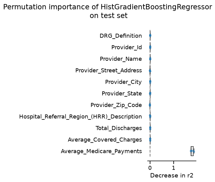
A final thing to be careful about is that SKD012 flags most provider fields and Total_Discharges as useless. As we can see in the importance plot below, every feature looks weak next to the golden billing column, even though some of them may recover once we drop it. We will keep them for now.

_ = first_report.inspection.permutation_importance().plot()


# SKD011 - Inspect after dropping golden feature
# ==============================================
#
# First let's evaluate the same model on the same test set with the payment features
# removed, and compare it with our original model.
#
# Thankfully there is still signal in the remaining features, as we get a decent R²
# of 0.89.

from skore import compare

X_without_payment = X.drop(
    columns=["Average_Medicare_Payments", "Average_Covered_Charges"]
)

second_report = evaluate(
    model,
    X=X_without_payment,
    y=y,
    splitter=splitter,
)

comparison = compare(
    {
        "with_payment_features": first_report,
        "without_payment_features": second_report,
    }
)
comparison.metrics.summarize().frame()

estimator	with_payment_features	without_payment_features
metric
r2	0.968625	0.890437
rmse	1236.859022	2311.336441
mae	555.159914	1318.776062
mape	0.052583	0.138348
fit_time	2.457898	2.374167
predict_time	0.232536	0.224389

Let us inspect which features are now the ones our model relies on the most. We can see that DRG_Definition is by far most important one, according to permutation importance. This feature encodes the medical reason for which patients were treated. It will therefore be available at inference time and we can use it.

_ = second_report.inspection.permutation_importance().plot()

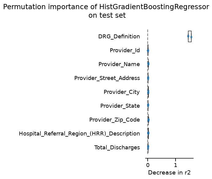
SKD012 now flags Provider_Id and Total_Discharges. Those look genuinely weak once billing leakage is gone: an identifier and a discharge count that barely moves the score. Other provider fields recovered some signal, which is why we did not treat the leaky SKD012 list as columns to drop.

The check still only sees original columns. TableVectorizer creates extra components from high-cardinality strings that can be weak too; we prune those next.

second_report.checks.summarize()

SKD012 - prune weak features inside the pipeline

SKD012 flagged Provider_Id and Total_Discharges on the original columns. It does not see the extra components TableVectorizer builds from high-cardinality fields such as DRG_Definition and provider names; some of those add little once the useful ones are present. We therefore select after vectorizing, with SelectFromModel, so the choice is fit on the training fold only.

Histogram gradient boosting has no feature_importances_, so the selector uses GradientBoostingRegressor. The final estimator stays a HistGradientBoostingRegressor on the reduced matrix.

from sklearn.ensemble import GradientBoostingRegressor
from sklearn.feature_selection import SelectFromModel

model_reduced = make_pipeline(
    vectorizer,
    SelectFromModel(
        GradientBoostingRegressor(random_state=42),
        threshold="median",
    ),
    regressor,
)
model_reduced

Pipeline(steps=[('tablevectorizer',
                 TableVectorizer(high_cardinality=StringEncoder(random_state=42))),
                ('selectfrommodel',
                 SelectFromModel(estimator=GradientBoostingRegressor(random_state=42),
                                 threshold='median')),
                ('histgradientboostingregressor',
                 HistGradientBoostingRegressor(random_state=42))])

In a Jupyter environment, please rerun this cell to show the HTML representation or trust the notebook.
On GitHub, the HTML representation is unable to render, please try loading this page with nbviewer.org.

Let us evaluate the reduced pipeline on the same split. Test scores are a on par, and the model is lighter: selection dropped the weak vectorized components before fitting histogram boosting.

third_report = evaluate(
    model_reduced,
    X=X_without_payment,
    y=y,
    splitter=splitter,
)

comparison_reduced = compare(
    {
        "without_payment_features": second_report,
        "without_payment_features_reduced": third_report,
    }
)
comparison_reduced.metrics.summarize().frame()

estimator	without_payment_features	without_payment_features_reduced
metric
r2	0.890437	0.890613
rmse	2311.336441	2309.483190
mae	1318.776062	1316.978826
mape	0.138348	0.138346
fit_time	2.374167	7.935268
predict_time	0.224389	0.134846

Conclusion

SKD011 and SKD012 often appear together when one leaky column dominates. Audit that column and compare with-and-without it; do not treat SKD012 flags on a leaky report as a drop list. Once leakage is gone, SKD012 may still flag identifiers or weak columns (Provider_Id, Total_Discharges here) while TableVectorizer also builds weak encoded components. Prune those inside the pipeline, for example with SelectFromModel, and check that test performance is preserved.