

Note
Go to the end to download the full example code.
SKD004 - High class imbalance#
SKD004 flags a binary classification task when the majority class exceeds 80 % of rows. Accuracy can look high while the minority class is ignored as a default. This notebook is mostly about how to work with that imbalance once the check fires: we do not try to make SKD004 disappear, because natural prevalence is often the right thing to keep.
What we do instead (see also Automated checks):
report absolute counts as well as percentages,
evaluate ranking and calibration (ROC AUC, log-loss) before trusting thresholded precision / recall,
tune the decision threshold under an explicit precision / recall or cost constraint (for example with
TunedThresholdClassifierCV),avoid
class_weightand resampling when calibrated probabilities matter,correct for prevalence shift if you collect minority-only data.
We use Covertype forest types 2 (majority) vs 5 (minority) on an 8,000-row stratified subsample. The goal is to keep natural prevalence, judge probability quality first, then choose a cut-off that matches the precision / recall trade-off you care about.
Load Covertype (types 2 vs 5)#
Types 2 vs 5 give a natural imbalance (type 2 is the majority class). We keep minority type 5 as the positive class and draw an 8,000-row stratified subsample so the gallery stays fast while absolute minority counts remain large enough to learn from.
import numpy as np
from sklearn.datasets import fetch_covtype
from sklearn.model_selection import train_test_split

df = fetch_covtype(as_frame=True).frame
pair = df.query("Cover_Type.isin([2, 5])")
y_full = (pair["Cover_Type"] == 5).astype(int).rename("is_type_5")
X_full = pair.drop(columns=["Cover_Type"])

X, _, y, _ = train_test_split(
    X_full,
    y_full,
    train_size=8_000,
    stratify=y_full,
    random_state=42,
)
y.value_counts(normalize=True).round(4)
is_type_5
0    0.9676
1    0.0324
Name: proportion, dtype: float64
is_type_5
0    7741
1     259
Name: count, dtype: int64
Inspect the feature matrix with TableReport.
from skrub import TableReport

TableReport(X)
| Elevation | Aspect | Slope | Horizontal_Distance_To_Hydrology | Vertical_Distance_To_Hydrology | Horizontal_Distance_To_Roadways | Hillshade_9am | Hillshade_Noon | Hillshade_3pm | Horizontal_Distance_To_Fire_Points | Wilderness_Area_0 | Wilderness_Area_1 | Wilderness_Area_2 | Wilderness_Area_3 | Soil_Type_0 | Soil_Type_1 | Soil_Type_2 | Soil_Type_3 | Soil_Type_4 | Soil_Type_5 | Soil_Type_6 | Soil_Type_7 | Soil_Type_8 | Soil_Type_9 | Soil_Type_10 | Soil_Type_11 | Soil_Type_12 | Soil_Type_13 | Soil_Type_14 | Soil_Type_15 | Soil_Type_16 | Soil_Type_17 | Soil_Type_18 | Soil_Type_19 | Soil_Type_20 | Soil_Type_21 | Soil_Type_22 | Soil_Type_23 | Soil_Type_24 | Soil_Type_25 | Soil_Type_26 | Soil_Type_27 | Soil_Type_28 | Soil_Type_29 | Soil_Type_30 | Soil_Type_31 | Soil_Type_32 | Soil_Type_33 | Soil_Type_34 | Soil_Type_35 | Soil_Type_36 | Soil_Type_37 | Soil_Type_38 | Soil_Type_39 | |
|---|---|---|---|---|---|---|---|---|---|---|---|---|---|---|---|---|---|---|---|---|---|---|---|---|---|---|---|---|---|---|---|---|---|---|---|---|---|---|---|---|---|---|---|---|---|---|---|---|---|---|---|---|---|---|
| 213,147 | 3.05e+03 | 21.0 | 8.00 | 124. | 15.0 | 1.23e+03 | 215. | 223. | 145. | 2.34e+03 | 1.00 | 0.00 | 0.00 | 0.00 | 0.00 | 0.00 | 0.00 | 0.00 | 0.00 | 0.00 | 0.00 | 0.00 | 0.00 | 0.00 | 0.00 | 0.00 | 0.00 | 0.00 | 0.00 | 0.00 | 0.00 | 0.00 | 0.00 | 0.00 | 0.00 | 0.00 | 0.00 | 0.00 | 0.00 | 0.00 | 0.00 | 0.00 | 1.00 | 0.00 | 0.00 | 0.00 | 0.00 | 0.00 | 0.00 | 0.00 | 0.00 | 0.00 | 0.00 | 0.00 |
| 109,197 | 2.61e+03 | 45.0 | 2.00 | 42.0 | -1.00 | 755. | 219. | 235. | 152. | 1.62e+03 | 1.00 | 0.00 | 0.00 | 0.00 | 0.00 | 0.00 | 0.00 | 0.00 | 0.00 | 0.00 | 0.00 | 0.00 | 0.00 | 0.00 | 0.00 | 1.00 | 0.00 | 0.00 | 0.00 | 0.00 | 0.00 | 0.00 | 0.00 | 0.00 | 0.00 | 0.00 | 0.00 | 0.00 | 0.00 | 0.00 | 0.00 | 0.00 | 0.00 | 0.00 | 0.00 | 0.00 | 0.00 | 0.00 | 0.00 | 0.00 | 0.00 | 0.00 | 0.00 | 0.00 |
| 171,741 | 2.99e+03 | 102. | 19.0 | 258. | 53.0 | 2.19e+03 | 248. | 212. | 86.0 | 911. | 1.00 | 0.00 | 0.00 | 0.00 | 0.00 | 0.00 | 0.00 | 0.00 | 0.00 | 0.00 | 0.00 | 0.00 | 0.00 | 0.00 | 0.00 | 0.00 | 0.00 | 0.00 | 0.00 | 0.00 | 0.00 | 0.00 | 0.00 | 0.00 | 0.00 | 0.00 | 0.00 | 0.00 | 0.00 | 0.00 | 0.00 | 0.00 | 0.00 | 1.00 | 0.00 | 0.00 | 0.00 | 0.00 | 0.00 | 0.00 | 0.00 | 0.00 | 0.00 | 0.00 |
| 361,152 | 2.98e+03 | 268. | 22.0 | 579. | 328. | 1.87e+03 | 156. | 242. | 221. | 1.68e+03 | 0.00 | 0.00 | 1.00 | 0.00 | 0.00 | 0.00 | 0.00 | 0.00 | 0.00 | 0.00 | 0.00 | 0.00 | 0.00 | 0.00 | 0.00 | 0.00 | 0.00 | 0.00 | 0.00 | 0.00 | 0.00 | 0.00 | 0.00 | 0.00 | 0.00 | 0.00 | 0.00 | 0.00 | 0.00 | 0.00 | 0.00 | 0.00 | 0.00 | 0.00 | 0.00 | 0.00 | 1.00 | 0.00 | 0.00 | 0.00 | 0.00 | 0.00 | 0.00 | 0.00 |
| 164,253 | 2.90e+03 | 78.0 | 6.00 | 170. | 0.00 | 1.35e+03 | 227. | 230. | 137. | 1.95e+03 | 1.00 | 0.00 | 0.00 | 0.00 | 0.00 | 0.00 | 0.00 | 0.00 | 0.00 | 0.00 | 0.00 | 0.00 | 0.00 | 0.00 | 0.00 | 0.00 | 0.00 | 0.00 | 0.00 | 0.00 | 0.00 | 0.00 | 0.00 | 0.00 | 0.00 | 0.00 | 0.00 | 0.00 | 0.00 | 0.00 | 0.00 | 0.00 | 1.00 | 0.00 | 0.00 | 0.00 | 0.00 | 0.00 | 0.00 | 0.00 | 0.00 | 0.00 | 0.00 | 0.00 |
| 58,342 | 2.64e+03 | 124. | 20.0 | 210. | 43.0 | 1.16e+03 | 249. | 221. | 91.0 | 2.32e+03 | 1.00 | 0.00 | 0.00 | 0.00 | 0.00 | 0.00 | 0.00 | 0.00 | 0.00 | 0.00 | 0.00 | 0.00 | 0.00 | 0.00 | 0.00 | 0.00 | 0.00 | 0.00 | 0.00 | 0.00 | 0.00 | 0.00 | 0.00 | 0.00 | 0.00 | 0.00 | 0.00 | 0.00 | 0.00 | 0.00 | 0.00 | 0.00 | 0.00 | 1.00 | 0.00 | 0.00 | 0.00 | 0.00 | 0.00 | 0.00 | 0.00 | 0.00 | 0.00 | 0.00 |
| 11,757 | 2.76e+03 | 60.0 | 25.0 | 258. | 81.0 | 277. | 231. | 180. | 68.0 | 1.87e+03 | 1.00 | 0.00 | 0.00 | 0.00 | 0.00 | 0.00 | 0.00 | 0.00 | 0.00 | 0.00 | 0.00 | 0.00 | 0.00 | 0.00 | 0.00 | 0.00 | 0.00 | 0.00 | 0.00 | 0.00 | 0.00 | 0.00 | 0.00 | 0.00 | 0.00 | 0.00 | 0.00 | 0.00 | 0.00 | 0.00 | 0.00 | 0.00 | 1.00 | 0.00 | 0.00 | 0.00 | 0.00 | 0.00 | 0.00 | 0.00 | 0.00 | 0.00 | 0.00 | 0.00 |
| 417,010 | 3.06e+03 | 244. | 24.0 | 108. | 33.0 | 2.51e+03 | 165. | 250. | 217. | 1.47e+03 | 0.00 | 0.00 | 1.00 | 0.00 | 0.00 | 0.00 | 0.00 | 0.00 | 0.00 | 0.00 | 0.00 | 0.00 | 0.00 | 0.00 | 0.00 | 0.00 | 0.00 | 0.00 | 0.00 | 0.00 | 0.00 | 0.00 | 0.00 | 0.00 | 0.00 | 0.00 | 1.00 | 0.00 | 0.00 | 0.00 | 0.00 | 0.00 | 0.00 | 0.00 | 0.00 | 0.00 | 0.00 | 0.00 | 0.00 | 0.00 | 0.00 | 0.00 | 0.00 | 0.00 |
| 258,803 | 3.01e+03 | 95.0 | 14.0 | 127. | 26.0 | 418. | 241. | 219. | 104. | 1.38e+03 | 0.00 | 0.00 | 1.00 | 0.00 | 0.00 | 0.00 | 0.00 | 0.00 | 0.00 | 0.00 | 0.00 | 0.00 | 0.00 | 0.00 | 0.00 | 0.00 | 0.00 | 0.00 | 0.00 | 0.00 | 0.00 | 0.00 | 0.00 | 0.00 | 0.00 | 0.00 | 0.00 | 0.00 | 0.00 | 0.00 | 0.00 | 0.00 | 0.00 | 0.00 | 0.00 | 1.00 | 0.00 | 0.00 | 0.00 | 0.00 | 0.00 | 0.00 | 0.00 | 0.00 |
| 304,052 | 2.96e+03 | 73.0 | 13.0 | 42.0 | 2.00 | 2.41e+03 | 235. | 214. | 108. | 1.85e+03 | 0.00 | 0.00 | 1.00 | 0.00 | 0.00 | 0.00 | 0.00 | 0.00 | 0.00 | 0.00 | 0.00 | 0.00 | 0.00 | 0.00 | 0.00 | 0.00 | 0.00 | 0.00 | 0.00 | 0.00 | 0.00 | 0.00 | 0.00 | 0.00 | 0.00 | 0.00 | 0.00 | 0.00 | 0.00 | 0.00 | 0.00 | 0.00 | 0.00 | 0.00 | 0.00 | 1.00 | 0.00 | 0.00 | 0.00 | 0.00 | 0.00 | 0.00 | 0.00 | 0.00 |
Elevation
Float64DType- Null values
- 0 (0.0%)
- Unique values
-
906 (11.3%)
This column has a high cardinality (> 40).
- Mean ± Std
- 2.91e+03 ± 187.
- Median ± IQR
- 2.93e+03 ± 250.
- Min | Max
- 2.15e+03 | 3.40e+03
Aspect
Float64DType- Null values
- 0 (0.0%)
- Unique values
-
361 (4.5%)
This column has a high cardinality (> 40).
- Mean ± Std
- 151. ± 107.
- Median ± IQR
- 126. ± 175.
- Min | Max
- 0.00 | 360.
Slope
Float64DType- Null values
- 0 (0.0%)
- Unique values
-
44 (0.5%)
This column has a high cardinality (> 40).
- Mean ± Std
- 13.7 ± 7.06
- Median ± IQR
- 13.0 ± 9.00
- Min | Max
- 0.00 | 45.0
Horizontal_Distance_To_Hydrology
Float64DType- Null values
- 0 (0.0%)
- Unique values
-
341 (4.3%)
This column has a high cardinality (> 40).
- Mean ± Std
- 276. ± 206.
- Median ± IQR
- 240. ± 270.
- Min | Max
- 0.00 | 1.37e+03
Vertical_Distance_To_Hydrology
Float64DType- Null values
- 0 (0.0%)
- Unique values
-
383 (4.8%)
This column has a high cardinality (> 40).
- Mean ± Std
- 45.5 ± 56.4
- Median ± IQR
- 30.0 ± 57.0
- Min | Max
- -153. | 549.
Horizontal_Distance_To_Roadways
Float64DType- Null values
- 0 (0.0%)
- Unique values
-
3,199 (40.0%)
This column has a high cardinality (> 40).
- Mean ± Std
- 2.36e+03 ± 1.60e+03
- Median ± IQR
- 1.97e+03 ± 2.18e+03
- Min | Max
- 30.0 | 6.94e+03
Hillshade_9am
Float64DType- Null values
- 0 (0.0%)
- Unique values
-
152 (1.9%)
This column has a high cardinality (> 40).
- Mean ± Std
- 214. ± 24.7
- Median ± IQR
- 220. ± 32.0
- Min | Max
- 84.0 | 254.
Hillshade_Noon
Float64DType- Null values
- 0 (0.0%)
- Unique values
-
114 (1.4%)
This column has a high cardinality (> 40).
- Mean ± Std
- 225. ± 18.6
- Median ± IQR
- 227. ± 24.0
- Min | Max
- 124. | 254.
Hillshade_3pm
Float64DType- Null values
- 0 (0.0%)
- Unique values
-
231 (2.9%)
This column has a high cardinality (> 40).
- Mean ± Std
- 142. ± 36.5
- Median ± IQR
- 142. ± 46.0
- Min | Max
- 0.00 | 251.
Horizontal_Distance_To_Fire_Points
Float64DType- Null values
- 0 (0.0%)
- Unique values
-
2,841 (35.5%)
This column has a high cardinality (> 40).
- Mean ± Std
- 2.14e+03 ± 1.40e+03
- Median ± IQR
- 1.83e+03 ± 1.46e+03
- Min | Max
- 30.0 | 7.08e+03
Wilderness_Area_0
Float64DType- Null values
- 0 (0.0%)
- Unique values
- 2 (< 0.1%)
- Mean ± Std
- 0.504 ± 0.500
- Median ± IQR
- 1.00 ± 1.00
- Min | Max
- 0.00 | 1.00
Wilderness_Area_1
Float64DType- Null values
- 0 (0.0%)
- Unique values
- 2 (< 0.1%)
- Mean ± Std
- 0.0319 ± 0.176
- Median ± IQR
- 0.00 ± 0.00
- Min | Max
- 0.00 | 1.00
Wilderness_Area_2
Float64DType- Null values
- 0 (0.0%)
- Unique values
- 2 (< 0.1%)
- Mean ± Std
- 0.451 ± 0.498
- Median ± IQR
- 0.00 ± 1.00
- Min | Max
- 0.00 | 1.00
Wilderness_Area_3
Float64DType- Null values
- 0 (0.0%)
- Unique values
- 2 (< 0.1%)
- Mean ± Std
- 0.0123 ± 0.110
- Median ± IQR
- 0.00 ± 0.00
- Min | Max
- 0.00 | 1.00
Soil_Type_0
Float64DType- Null values
- 0 (0.0%)
Soil_Type_1
Float64DType- Null values
- 0 (0.0%)
- Unique values
- 2 (< 0.1%)
- Mean ± Std
- 0.00500 ± 0.0705
- Median ± IQR
- 0.00 ± 0.00
- Min | Max
- 0.00 | 1.00
Soil_Type_2
Float64DType- Null values
- 0 (0.0%)
- Unique values
- 2 (< 0.1%)
- Mean ± Std
- 0.00413 ± 0.0641
- Median ± IQR
- 0.00 ± 0.00
- Min | Max
- 0.00 | 1.00
Soil_Type_3
Float64DType- Null values
- 0 (0.0%)
- Unique values
- 2 (< 0.1%)
- Mean ± Std
- 0.0140 ± 0.117
- Median ± IQR
- 0.00 ± 0.00
- Min | Max
- 0.00 | 1.00
Soil_Type_4
Float64DType- Null values
- 0 (0.0%)
Soil_Type_5
Float64DType- Null values
- 0 (0.0%)
- Unique values
- 2 (< 0.1%)
- Mean ± Std
- 0.00387 ± 0.0621
- Median ± IQR
- 0.00 ± 0.00
- Min | Max
- 0.00 | 1.00
Soil_Type_6
Float64DType- Null values
- 0 (0.0%)
- Unique values
- 2 (< 0.1%)
- Mean ± Std
- 0.000375 ± 0.0194
- Median ± IQR
- 0.00 ± 0.00
- Min | Max
- 0.00 | 1.00
Soil_Type_7
Float64DType- Null values
- 0 (0.0%)
- Unique values
- 2 (< 0.1%)
- Mean ± Std
- 0.000375 ± 0.0194
- Median ± IQR
- 0.00 ± 0.00
- Min | Max
- 0.00 | 1.00
Soil_Type_8
Float64DType- Null values
- 0 (0.0%)
- Unique values
- 2 (< 0.1%)
- Mean ± Std
- 0.00275 ± 0.0524
- Median ± IQR
- 0.00 ± 0.00
- Min | Max
- 0.00 | 1.00
Soil_Type_9
Float64DType- Null values
- 0 (0.0%)
- Unique values
- 2 (< 0.1%)
- Mean ± Std
- 0.0413 ± 0.199
- Median ± IQR
- 0.00 ± 0.00
- Min | Max
- 0.00 | 1.00
Soil_Type_10
Float64DType- Null values
- 0 (0.0%)
- Unique values
- 2 (< 0.1%)
- Mean ± Std
- 0.0318 ± 0.175
- Median ± IQR
- 0.00 ± 0.00
- Min | Max
- 0.00 | 1.00
Soil_Type_11
Float64DType- Null values
- 0 (0.0%)
- Unique values
- 2 (< 0.1%)
- Mean ± Std
- 0.0909 ± 0.287
- Median ± IQR
- 0.00 ± 0.00
- Min | Max
- 0.00 | 1.00
Soil_Type_12
Float64DType- Null values
- 0 (0.0%)
- Unique values
- 2 (< 0.1%)
- Mean ± Std
- 0.0480 ± 0.214
- Median ± IQR
- 0.00 ± 0.00
- Min | Max
- 0.00 | 1.00
Soil_Type_13
Float64DType- Null values
- 0 (0.0%)
Soil_Type_14
Float64DType- Null values
- 0 (0.0%)
Soil_Type_15
Float64DType- Null values
- 0 (0.0%)
- Unique values
- 2 (< 0.1%)
- Mean ± Std
- 0.00550 ± 0.0740
- Median ± IQR
- 0.00 ± 0.00
- Min | Max
- 0.00 | 1.00
Soil_Type_16
Float64DType- Null values
- 0 (0.0%)
- Unique values
- 2 (< 0.1%)
- Mean ± Std
- 0.00537 ± 0.0731
- Median ± IQR
- 0.00 ± 0.00
- Min | Max
- 0.00 | 1.00
Soil_Type_17
Float64DType- Null values
- 0 (0.0%)
- Unique values
- 2 (< 0.1%)
- Mean ± Std
- 0.00675 ± 0.0819
- Median ± IQR
- 0.00 ± 0.00
- Min | Max
- 0.00 | 1.00
Soil_Type_18
Float64DType- Null values
- 0 (0.0%)
- Unique values
- 2 (< 0.1%)
- Mean ± Std
- 0.00500 ± 0.0705
- Median ± IQR
- 0.00 ± 0.00
- Min | Max
- 0.00 | 1.00
Soil_Type_19
Float64DType- Null values
- 0 (0.0%)
- Unique values
- 2 (< 0.1%)
- Mean ± Std
- 0.0181 ± 0.133
- Median ± IQR
- 0.00 ± 0.00
- Min | Max
- 0.00 | 1.00
Soil_Type_20
Float64DType- Null values
- 0 (0.0%)
Soil_Type_21
Float64DType- Null values
- 0 (0.0%)
- Unique values
- 2 (< 0.1%)
- Mean ± Std
- 0.0238 ± 0.152
- Median ± IQR
- 0.00 ± 0.00
- Min | Max
- 0.00 | 1.00
Soil_Type_22
Float64DType- Null values
- 0 (0.0%)
- Unique values
- 2 (< 0.1%)
- Mean ± Std
- 0.0729 ± 0.260
- Median ± IQR
- 0.00 ± 0.00
- Min | Max
- 0.00 | 1.00
Soil_Type_23
Float64DType- Null values
- 0 (0.0%)
- Unique values
- 2 (< 0.1%)
- Mean ± Std
- 0.0338 ± 0.181
- Median ± IQR
- 0.00 ± 0.00
- Min | Max
- 0.00 | 1.00
Soil_Type_24
Float64DType- Null values
- 0 (0.0%)
- Unique values
- 2 (< 0.1%)
- Mean ± Std
- 0.00125 ± 0.0353
- Median ± IQR
- 0.00 ± 0.00
- Min | Max
- 0.00 | 1.00
Soil_Type_25
Float64DType- Null values
- 0 (0.0%)
- Unique values
- 2 (< 0.1%)
- Mean ± Std
- 0.00750 ± 0.0863
- Median ± IQR
- 0.00 ± 0.00
- Min | Max
- 0.00 | 1.00
Soil_Type_26
Float64DType- Null values
- 0 (0.0%)
- Unique values
- 2 (< 0.1%)
- Mean ± Std
- 0.00112 ± 0.0335
- Median ± IQR
- 0.00 ± 0.00
- Min | Max
- 0.00 | 1.00
Soil_Type_27
Float64DType- Null values
- 0 (0.0%)
- Unique values
- 2 (< 0.1%)
- Mean ± Std
- 0.00350 ± 0.0591
- Median ± IQR
- 0.00 ± 0.00
- Min | Max
- 0.00 | 1.00
Soil_Type_28
Float64DType- Null values
- 0 (0.0%)
- Unique values
- 2 (< 0.1%)
- Mean ± Std
- 0.250 ± 0.433
- Median ± IQR
- 0.00 ± 1.00
- Min | Max
- 0.00 | 1.00
Soil_Type_29
Float64DType- Null values
- 0 (0.0%)
- Unique values
- 2 (< 0.1%)
- Mean ± Std
- 0.0744 ± 0.262
- Median ± IQR
- 0.00 ± 0.00
- Min | Max
- 0.00 | 1.00
Soil_Type_30
Float64DType- Null values
- 0 (0.0%)
- Unique values
- 2 (< 0.1%)
- Mean ± Std
- 0.0467 ± 0.211
- Median ± IQR
- 0.00 ± 0.00
- Min | Max
- 0.00 | 1.00
Soil_Type_31
Float64DType- Null values
- 0 (0.0%)
- Unique values
- 2 (< 0.1%)
- Mean ± Std
- 0.105 ± 0.307
- Median ± IQR
- 0.00 ± 0.00
- Min | Max
- 0.00 | 1.00
Soil_Type_32
Float64DType- Null values
- 0 (0.0%)
- Unique values
- 2 (< 0.1%)
- Mean ± Std
- 0.0882 ± 0.284
- Median ± IQR
- 0.00 ± 0.00
- Min | Max
- 0.00 | 1.00
Soil_Type_33
Float64DType- Null values
- 0 (0.0%)
- Unique values
- 2 (< 0.1%)
- Mean ± Std
- 0.00387 ± 0.0621
- Median ± IQR
- 0.00 ± 0.00
- Min | Max
- 0.00 | 1.00
Soil_Type_34
Float64DType- Null values
- 0 (0.0%)
Soil_Type_35
Float64DType- Null values
- 0 (0.0%)
Soil_Type_36
Float64DType- Null values
- 0 (0.0%)
Soil_Type_37
Float64DType- Null values
- 0 (0.0%)
- Unique values
- 2 (< 0.1%)
- Mean ± Std
- 0.00250 ± 0.0499
- Median ± IQR
- 0.00 ± 0.00
- Min | Max
- 0.00 | 1.00
Soil_Type_38
Float64DType- Null values
- 0 (0.0%)
- Unique values
- 2 (< 0.1%)
- Mean ± Std
- 0.000875 ± 0.0296
- Median ± IQR
- 0.00 ± 0.00
- Min | Max
- 0.00 | 1.00
Soil_Type_39
Float64DType- Null values
- 0 (0.0%)
- Unique values
- 2 (< 0.1%)
- Mean ± Std
- 0.00112 ± 0.0335
- Median ± IQR
- 0.00 ± 0.00
- Min | Max
- 0.00 | 1.00
No columns match the selected filter: . You can change the column filter in the dropdown menu above.
| Column | Column name | dtype | Is sorted | Null values | Unique values | Mean | Std | Min | Median | Max |
|---|---|---|---|---|---|---|---|---|---|---|
| 0 | Elevation | Float64DType | False | 0 (0.0%) | 906 (11.3%) | 2.91e+03 | 187. | 2.15e+03 | 2.93e+03 | 3.40e+03 |
| 1 | Aspect | Float64DType | False | 0 (0.0%) | 361 (4.5%) | 151. | 107. | 0.00 | 126. | 360. |
| 2 | Slope | Float64DType | False | 0 (0.0%) | 44 (0.5%) | 13.7 | 7.06 | 0.00 | 13.0 | 45.0 |
| 3 | Horizontal_Distance_To_Hydrology | Float64DType | False | 0 (0.0%) | 341 (4.3%) | 276. | 206. | 0.00 | 240. | 1.37e+03 |
| 4 | Vertical_Distance_To_Hydrology | Float64DType | False | 0 (0.0%) | 383 (4.8%) | 45.5 | 56.4 | -153. | 30.0 | 549. |
| 5 | Horizontal_Distance_To_Roadways | Float64DType | False | 0 (0.0%) | 3199 (40.0%) | 2.36e+03 | 1.60e+03 | 30.0 | 1.97e+03 | 6.94e+03 |
| 6 | Hillshade_9am | Float64DType | False | 0 (0.0%) | 152 (1.9%) | 214. | 24.7 | 84.0 | 220. | 254. |
| 7 | Hillshade_Noon | Float64DType | False | 0 (0.0%) | 114 (1.4%) | 225. | 18.6 | 124. | 227. | 254. |
| 8 | Hillshade_3pm | Float64DType | False | 0 (0.0%) | 231 (2.9%) | 142. | 36.5 | 0.00 | 142. | 251. |
| 9 | Horizontal_Distance_To_Fire_Points | Float64DType | False | 0 (0.0%) | 2841 (35.5%) | 2.14e+03 | 1.40e+03 | 30.0 | 1.83e+03 | 7.08e+03 |
| 10 | Wilderness_Area_0 | Float64DType | False | 0 (0.0%) | 2 (< 0.1%) | 0.504 | 0.500 | 0.00 | 1.00 | 1.00 |
| 11 | Wilderness_Area_1 | Float64DType | False | 0 (0.0%) | 2 (< 0.1%) | 0.0319 | 0.176 | 0.00 | 0.00 | 1.00 |
| 12 | Wilderness_Area_2 | Float64DType | False | 0 (0.0%) | 2 (< 0.1%) | 0.451 | 0.498 | 0.00 | 0.00 | 1.00 |
| 13 | Wilderness_Area_3 | Float64DType | False | 0 (0.0%) | 2 (< 0.1%) | 0.0123 | 0.110 | 0.00 | 0.00 | 1.00 |
| 14 | Soil_Type_0 | Float64DType | True | 0 (0.0%) | 1 (< 0.1%) | 0.00 | 0.00 | |||
| 15 | Soil_Type_1 | Float64DType | False | 0 (0.0%) | 2 (< 0.1%) | 0.00500 | 0.0705 | 0.00 | 0.00 | 1.00 |
| 16 | Soil_Type_2 | Float64DType | False | 0 (0.0%) | 2 (< 0.1%) | 0.00413 | 0.0641 | 0.00 | 0.00 | 1.00 |
| 17 | Soil_Type_3 | Float64DType | False | 0 (0.0%) | 2 (< 0.1%) | 0.0140 | 0.117 | 0.00 | 0.00 | 1.00 |
| 18 | Soil_Type_4 | Float64DType | True | 0 (0.0%) | 1 (< 0.1%) | 0.00 | 0.00 | |||
| 19 | Soil_Type_5 | Float64DType | False | 0 (0.0%) | 2 (< 0.1%) | 0.00387 | 0.0621 | 0.00 | 0.00 | 1.00 |
| 20 | Soil_Type_6 | Float64DType | False | 0 (0.0%) | 2 (< 0.1%) | 0.000375 | 0.0194 | 0.00 | 0.00 | 1.00 |
| 21 | Soil_Type_7 | Float64DType | False | 0 (0.0%) | 2 (< 0.1%) | 0.000375 | 0.0194 | 0.00 | 0.00 | 1.00 |
| 22 | Soil_Type_8 | Float64DType | False | 0 (0.0%) | 2 (< 0.1%) | 0.00275 | 0.0524 | 0.00 | 0.00 | 1.00 |
| 23 | Soil_Type_9 | Float64DType | False | 0 (0.0%) | 2 (< 0.1%) | 0.0413 | 0.199 | 0.00 | 0.00 | 1.00 |
| 24 | Soil_Type_10 | Float64DType | False | 0 (0.0%) | 2 (< 0.1%) | 0.0318 | 0.175 | 0.00 | 0.00 | 1.00 |
| 25 | Soil_Type_11 | Float64DType | False | 0 (0.0%) | 2 (< 0.1%) | 0.0909 | 0.287 | 0.00 | 0.00 | 1.00 |
| 26 | Soil_Type_12 | Float64DType | False | 0 (0.0%) | 2 (< 0.1%) | 0.0480 | 0.214 | 0.00 | 0.00 | 1.00 |
| 27 | Soil_Type_13 | Float64DType | True | 0 (0.0%) | 1 (< 0.1%) | 0.00 | 0.00 | |||
| 28 | Soil_Type_14 | Float64DType | True | 0 (0.0%) | 1 (< 0.1%) | 0.00 | 0.00 | |||
| 29 | Soil_Type_15 | Float64DType | False | 0 (0.0%) | 2 (< 0.1%) | 0.00550 | 0.0740 | 0.00 | 0.00 | 1.00 |
| 30 | Soil_Type_16 | Float64DType | False | 0 (0.0%) | 2 (< 0.1%) | 0.00537 | 0.0731 | 0.00 | 0.00 | 1.00 |
| 31 | Soil_Type_17 | Float64DType | False | 0 (0.0%) | 2 (< 0.1%) | 0.00675 | 0.0819 | 0.00 | 0.00 | 1.00 |
| 32 | Soil_Type_18 | Float64DType | False | 0 (0.0%) | 2 (< 0.1%) | 0.00500 | 0.0705 | 0.00 | 0.00 | 1.00 |
| 33 | Soil_Type_19 | Float64DType | False | 0 (0.0%) | 2 (< 0.1%) | 0.0181 | 0.133 | 0.00 | 0.00 | 1.00 |
| 34 | Soil_Type_20 | Float64DType | True | 0 (0.0%) | 1 (< 0.1%) | 0.00 | 0.00 | |||
| 35 | Soil_Type_21 | Float64DType | False | 0 (0.0%) | 2 (< 0.1%) | 0.0238 | 0.152 | 0.00 | 0.00 | 1.00 |
| 36 | Soil_Type_22 | Float64DType | False | 0 (0.0%) | 2 (< 0.1%) | 0.0729 | 0.260 | 0.00 | 0.00 | 1.00 |
| 37 | Soil_Type_23 | Float64DType | False | 0 (0.0%) | 2 (< 0.1%) | 0.0338 | 0.181 | 0.00 | 0.00 | 1.00 |
| 38 | Soil_Type_24 | Float64DType | False | 0 (0.0%) | 2 (< 0.1%) | 0.00125 | 0.0353 | 0.00 | 0.00 | 1.00 |
| 39 | Soil_Type_25 | Float64DType | False | 0 (0.0%) | 2 (< 0.1%) | 0.00750 | 0.0863 | 0.00 | 0.00 | 1.00 |
| 40 | Soil_Type_26 | Float64DType | False | 0 (0.0%) | 2 (< 0.1%) | 0.00112 | 0.0335 | 0.00 | 0.00 | 1.00 |
| 41 | Soil_Type_27 | Float64DType | False | 0 (0.0%) | 2 (< 0.1%) | 0.00350 | 0.0591 | 0.00 | 0.00 | 1.00 |
| 42 | Soil_Type_28 | Float64DType | False | 0 (0.0%) | 2 (< 0.1%) | 0.250 | 0.433 | 0.00 | 0.00 | 1.00 |
| 43 | Soil_Type_29 | Float64DType | False | 0 (0.0%) | 2 (< 0.1%) | 0.0744 | 0.262 | 0.00 | 0.00 | 1.00 |
| 44 | Soil_Type_30 | Float64DType | False | 0 (0.0%) | 2 (< 0.1%) | 0.0467 | 0.211 | 0.00 | 0.00 | 1.00 |
| 45 | Soil_Type_31 | Float64DType | False | 0 (0.0%) | 2 (< 0.1%) | 0.105 | 0.307 | 0.00 | 0.00 | 1.00 |
| 46 | Soil_Type_32 | Float64DType | False | 0 (0.0%) | 2 (< 0.1%) | 0.0882 | 0.284 | 0.00 | 0.00 | 1.00 |
| 47 | Soil_Type_33 | Float64DType | False | 0 (0.0%) | 2 (< 0.1%) | 0.00387 | 0.0621 | 0.00 | 0.00 | 1.00 |
| 48 | Soil_Type_34 | Float64DType | True | 0 (0.0%) | 1 (< 0.1%) | 0.00 | 0.00 | |||
| 49 | Soil_Type_35 | Float64DType | True | 0 (0.0%) | 1 (< 0.1%) | 0.00 | 0.00 | |||
| 50 | Soil_Type_36 | Float64DType | True | 0 (0.0%) | 1 (< 0.1%) | 0.00 | 0.00 | |||
| 51 | Soil_Type_37 | Float64DType | False | 0 (0.0%) | 2 (< 0.1%) | 0.00250 | 0.0499 | 0.00 | 0.00 | 1.00 |
| 52 | Soil_Type_38 | Float64DType | False | 0 (0.0%) | 2 (< 0.1%) | 0.000875 | 0.0296 | 0.00 | 0.00 | 1.00 |
| 53 | Soil_Type_39 | Float64DType | False | 0 (0.0%) | 2 (< 0.1%) | 0.00112 | 0.0335 | 0.00 | 0.00 | 1.00 |
No columns match the selected filter: . You can change the column filter in the dropdown menu above.
Plotting was skipped. This is due to either:
- The dataframe exceeding the configured
table_report_plots_thresholdlimit (default: 30). - The
plot_distributionsoption being set toFalse(default:"auto", which applies the configuredtable_report_plots_threshold).
You can adjust this behavior in several ways:
- To force plotting for a single report:
report = TableReport(df, plot_distributions=True) - To change the threshold for the current Python session, use
skrub.set_config:from skrub import set_config set_config(table_report_plots_threshold=50) - To make the change permanent, use an environment variable:
export SKB_TABLE_REPORT_PLOTS_THRESHOLD=50
No columns match the selected filter: . You can change the column filter in the dropdown menu above.
Computing pairwise associations was skipped. This is due to either:
- The dataframe exceeding the configured
table_report_associations_thresholdlimit (default: 30). - The
compute_associationsoption being set toFalse(default:"auto", which applies the configuredtable_report_associations_threshold).
You can adjust this behavior in several ways:
- To force computation for a single report:
report = TableReport(df, compute_associations=True) - To change the threshold for the current Python session, use
skrub.set_config:from skrub import set_config set_config(table_report_associations_threshold=50) - To make the change permanent, use an environment variable:
export SKB_TABLE_REPORT_ASSOCIATIONS_THRESHOLD=50
Please enable javascript
The skrub table reports need javascript to display correctly. If you are displaying a report in a Jupyter notebook and you see this message, you may need to re-execute the cell or to trust the notebook (button on the top right or "File > Trust notebook").
The binary target marks type-5 stands; the majority class exceeds 80 % of rows, so SKD004 will fire.
Trigger SKD004 - default classifier on imbalanced labels#
A default gradient boosting classifier does not change label counts. The check cares about the class mix in the data, not about whether we reweighted the loss.
from sklearn.ensemble import HistGradientBoostingClassifier
from skore import TrainTestSplit, evaluate

splitter = TrainTestSplit(test_size=0.2, random_state=42, stratify=y)
classifier = HistGradientBoostingClassifier(random_state=42)

report = evaluate(
    classifier,
    X=X,
    y=y,
    pos_label=1,
    splitter=splitter,
)
report
| Metric | HistGradientBoostingClassifier |
|---|---|
| Accuracy | 0.970625 |
| Precision | 0.608696 |
| Recall | 0.269231 |
| ROC AUC | 0.909586 |
| Log loss | 0.112095 |
| Brier score | 0.023782 |
| Fit time (s) | 0.751526 |
| Predict time (s) | 0.020438 |
- [SKD004] High class imbalance. Class [0] represents more than 80% of the dataset samples. Accuracy should not be used alone to assess model performance as it may be misleading by ignoring poor performance on the underrepresented class.
- [SKD008] Highly correlated input features. 1 pair(s) of features have a Spearman correlation above 0.9. Highly correlated features can destabilize linear model coefficients and feature-importance estimates, and may cause collinearity-induced numerical issues.Dropping redundant features may also improve model performance.
- [SKD016] Estimator not tuned. Estimator(s) left at default settings; consider tuning: ['learning_rate', 'max_leaf_nodes'] for HistGradientBoostingClassifier.
- [SKD003] Inconsistent performance across splits. Not applicable to estimator reports.
- [SKD005] Underrepresented classes. ML task is not multiclass classification. Got binary-classification.
- [SKD006] Coefficient interpretation. Estimator is not a linear model: it does not have a `coef_` attribute.
- [SKD007] MDI biased for high-cardinality features. Estimator is not a tree-based model: it does not have a `feature_importances_` attribute.
- [SKD013] Train-test overlap in time series. No datetime column found.
- [SKD014] Hyperparameters at search edge. Estimator is not a BaseSearchCV instance. Got HistGradientBoostingClassifier.
- [SKD015] Hyperparameters worth tuning. Estimator is not a BaseSearchCV instance. Got HistGradientBoostingClassifier.
No checks were muted.
Fast mode is on: expensive checks are skipped unless already cached.
Mute a check by passing its code to ignore, e.g. .checks.summarize(ignore=['SKD001']).
HistGradientBoostingClassifier(random_state=42)In a Jupyter environment, please rerun this cell to show the HTML representation or trust the notebook.
On GitHub, the HTML representation is unable to render, please try loading this page with nbviewer.org.
Parameters
Fitted attributes
| Elevation | Aspect | Slope | Horizontal_Distance_To_Hydrology | Vertical_Distance_To_Hydrology | Horizontal_Distance_To_Roadways | Hillshade_9am | Hillshade_Noon | Hillshade_3pm | Horizontal_Distance_To_Fire_Points | Wilderness_Area_0 | Wilderness_Area_1 | Wilderness_Area_2 | Wilderness_Area_3 | Soil_Type_0 | Soil_Type_1 | Soil_Type_2 | Soil_Type_3 | Soil_Type_4 | Soil_Type_5 | Soil_Type_6 | Soil_Type_7 | Soil_Type_8 | Soil_Type_9 | Soil_Type_10 | Soil_Type_11 | Soil_Type_12 | Soil_Type_13 | Soil_Type_14 | Soil_Type_15 | Soil_Type_16 | Soil_Type_17 | Soil_Type_18 | Soil_Type_19 | Soil_Type_20 | Soil_Type_21 | Soil_Type_22 | Soil_Type_23 | Soil_Type_24 | Soil_Type_25 | Soil_Type_26 | Soil_Type_27 | Soil_Type_28 | Soil_Type_29 | Soil_Type_30 | Soil_Type_31 | Soil_Type_32 | Soil_Type_33 | Soil_Type_34 | Soil_Type_35 | Soil_Type_36 | Soil_Type_37 | Soil_Type_38 | Soil_Type_39 | is_type_5 | |
|---|---|---|---|---|---|---|---|---|---|---|---|---|---|---|---|---|---|---|---|---|---|---|---|---|---|---|---|---|---|---|---|---|---|---|---|---|---|---|---|---|---|---|---|---|---|---|---|---|---|---|---|---|---|---|---|
| 0 | 2.83e+03 | 83.0 | 28.0 | 242. | 161. | 1.41e+03 | 246. | 178. | 42.0 | 1.02e+03 | 0.00 | 0.00 | 1.00 | 0.00 | 0.00 | 0.00 | 0.00 | 0.00 | 0.00 | 0.00 | 0.00 | 0.00 | 0.00 | 0.00 | 0.00 | 0.00 | 1.00 | 0.00 | 0.00 | 0.00 | 0.00 | 0.00 | 0.00 | 0.00 | 0.00 | 0.00 | 0.00 | 0.00 | 0.00 | 0.00 | 0.00 | 0.00 | 0.00 | 0.00 | 0.00 | 0.00 | 0.00 | 0.00 | 0.00 | 0.00 | 0.00 | 0.00 | 0.00 | 0.00 | 0 |
| 1 | 3.06e+03 | 232. | 8.00 | 721. | 26.0 | 6.20e+03 | 207. | 248. | 178. | 3.36e+03 | 1.00 | 0.00 | 0.00 | 0.00 | 0.00 | 0.00 | 0.00 | 0.00 | 0.00 | 0.00 | 0.00 | 0.00 | 0.00 | 0.00 | 0.00 | 0.00 | 0.00 | 0.00 | 0.00 | 0.00 | 0.00 | 0.00 | 0.00 | 0.00 | 0.00 | 0.00 | 0.00 | 0.00 | 0.00 | 0.00 | 0.00 | 0.00 | 1.00 | 0.00 | 0.00 | 0.00 | 0.00 | 0.00 | 0.00 | 0.00 | 0.00 | 0.00 | 0.00 | 0.00 | 0 |
| 2 | 2.93e+03 | 241. | 6.00 | 295. | 26.0 | 5.36e+03 | 209. | 245. | 174. | 4.47e+03 | 1.00 | 0.00 | 0.00 | 0.00 | 0.00 | 0.00 | 0.00 | 0.00 | 0.00 | 0.00 | 0.00 | 0.00 | 0.00 | 0.00 | 0.00 | 0.00 | 0.00 | 0.00 | 0.00 | 0.00 | 0.00 | 0.00 | 0.00 | 0.00 | 0.00 | 0.00 | 1.00 | 0.00 | 0.00 | 0.00 | 0.00 | 0.00 | 0.00 | 0.00 | 0.00 | 0.00 | 0.00 | 0.00 | 0.00 | 0.00 | 0.00 | 0.00 | 0.00 | 0.00 | 0 |
| 3 | 2.93e+03 | 296. | 7.00 | 382. | 53.0 | 3.74e+03 | 200. | 238. | 178. | 5.35e+03 | 1.00 | 0.00 | 0.00 | 0.00 | 0.00 | 0.00 | 0.00 | 0.00 | 0.00 | 0.00 | 0.00 | 0.00 | 0.00 | 0.00 | 0.00 | 0.00 | 0.00 | 0.00 | 0.00 | 0.00 | 0.00 | 0.00 | 0.00 | 0.00 | 0.00 | 0.00 | 0.00 | 0.00 | 0.00 | 0.00 | 0.00 | 0.00 | 1.00 | 0.00 | 0.00 | 0.00 | 0.00 | 0.00 | 0.00 | 0.00 | 0.00 | 0.00 | 0.00 | 0.00 | 0 |
| 4 | 2.91e+03 | 325. | 6.00 | 319. | 67.0 | 3.15e+03 | 206. | 234. | 167. | 2.27e+03 | 1.00 | 0.00 | 0.00 | 0.00 | 0.00 | 0.00 | 0.00 | 0.00 | 0.00 | 0.00 | 0.00 | 0.00 | 0.00 | 0.00 | 0.00 | 1.00 | 0.00 | 0.00 | 0.00 | 0.00 | 0.00 | 0.00 | 0.00 | 0.00 | 0.00 | 0.00 | 0.00 | 0.00 | 0.00 | 0.00 | 0.00 | 0.00 | 0.00 | 0.00 | 0.00 | 0.00 | 0.00 | 0.00 | 0.00 | 0.00 | 0.00 | 0.00 | 0.00 | 0.00 | 0 |
| 7,995 | 3.08e+03 | 145. | 19.0 | 268. | 67.0 | 735. | 243. | 233. | 111. | 1.37e+03 | 0.00 | 0.00 | 1.00 | 0.00 | 0.00 | 0.00 | 0.00 | 0.00 | 0.00 | 0.00 | 0.00 | 0.00 | 0.00 | 0.00 | 0.00 | 0.00 | 0.00 | 0.00 | 0.00 | 0.00 | 0.00 | 0.00 | 0.00 | 0.00 | 0.00 | 0.00 | 1.00 | 0.00 | 0.00 | 0.00 | 0.00 | 0.00 | 0.00 | 0.00 | 0.00 | 0.00 | 0.00 | 0.00 | 0.00 | 0.00 | 0.00 | 0.00 | 0.00 | 0.00 | 0 |
| 7,996 | 2.97e+03 | 167. | 17.0 | 306. | 42.0 | 2.32e+03 | 231. | 244. | 138. | 1.54e+03 | 0.00 | 0.00 | 1.00 | 0.00 | 0.00 | 0.00 | 0.00 | 0.00 | 0.00 | 0.00 | 0.00 | 0.00 | 0.00 | 0.00 | 0.00 | 0.00 | 1.00 | 0.00 | 0.00 | 0.00 | 0.00 | 0.00 | 0.00 | 0.00 | 0.00 | 0.00 | 0.00 | 0.00 | 0.00 | 0.00 | 0.00 | 0.00 | 0.00 | 0.00 | 0.00 | 0.00 | 0.00 | 0.00 | 0.00 | 0.00 | 0.00 | 0.00 | 0.00 | 0.00 | 0 |
| 7,997 | 2.53e+03 | 41.0 | 5.00 | 210. | 22.0 | 787. | 221. | 228. | 143. | 960. | 0.00 | 0.00 | 0.00 | 1.00 | 0.00 | 0.00 | 0.00 | 0.00 | 0.00 | 1.00 | 0.00 | 0.00 | 0.00 | 0.00 | 0.00 | 0.00 | 0.00 | 0.00 | 0.00 | 0.00 | 0.00 | 0.00 | 0.00 | 0.00 | 0.00 | 0.00 | 0.00 | 0.00 | 0.00 | 0.00 | 0.00 | 0.00 | 0.00 | 0.00 | 0.00 | 0.00 | 0.00 | 0.00 | 0.00 | 0.00 | 0.00 | 0.00 | 0.00 | 0.00 | 0 |
| 7,998 | 2.66e+03 | 93.0 | 14.0 | 390. | 94.0 | 1.30e+03 | 241. | 218. | 104. | 722. | 1.00 | 0.00 | 0.00 | 0.00 | 0.00 | 0.00 | 0.00 | 0.00 | 0.00 | 0.00 | 0.00 | 0.00 | 0.00 | 0.00 | 0.00 | 0.00 | 0.00 | 0.00 | 0.00 | 0.00 | 0.00 | 0.00 | 0.00 | 0.00 | 0.00 | 0.00 | 0.00 | 0.00 | 0.00 | 0.00 | 0.00 | 0.00 | 1.00 | 0.00 | 0.00 | 0.00 | 0.00 | 0.00 | 0.00 | 0.00 | 0.00 | 0.00 | 0.00 | 0.00 | 0 |
| 7,999 | 3.17e+03 | 247. | 23.0 | 534. | 102. | 6.03e+03 | 166. | 250. | 217. | 1.83e+03 | 1.00 | 0.00 | 0.00 | 0.00 | 0.00 | 0.00 | 0.00 | 0.00 | 0.00 | 0.00 | 0.00 | 0.00 | 0.00 | 0.00 | 0.00 | 0.00 | 0.00 | 0.00 | 0.00 | 0.00 | 0.00 | 0.00 | 0.00 | 0.00 | 0.00 | 0.00 | 0.00 | 0.00 | 0.00 | 0.00 | 0.00 | 0.00 | 0.00 | 1.00 | 0.00 | 0.00 | 0.00 | 0.00 | 0.00 | 0.00 | 0.00 | 0.00 | 0.00 | 0.00 | 0 |
Elevation
Float64DType- Null values
- 0 (0.0%)
- Unique values
-
906 (11.3%)
This column has a high cardinality (> 40).
- Mean ± Std
- 2.91e+03 ± 187.
- Median ± IQR
- 2.93e+03 ± 250.
- Min | Max
- 2.15e+03 | 3.40e+03
Aspect
Float64DType- Null values
- 0 (0.0%)
- Unique values
-
361 (4.5%)
This column has a high cardinality (> 40).
- Mean ± Std
- 151. ± 107.
- Median ± IQR
- 126. ± 175.
- Min | Max
- 0.00 | 360.
Slope
Float64DType- Null values
- 0 (0.0%)
- Unique values
-
44 (0.5%)
This column has a high cardinality (> 40).
- Mean ± Std
- 13.7 ± 7.06
- Median ± IQR
- 13.0 ± 9.00
- Min | Max
- 0.00 | 45.0
Horizontal_Distance_To_Hydrology
Float64DType- Null values
- 0 (0.0%)
- Unique values
-
341 (4.3%)
This column has a high cardinality (> 40).
- Mean ± Std
- 276. ± 206.
- Median ± IQR
- 240. ± 270.
- Min | Max
- 0.00 | 1.37e+03
Vertical_Distance_To_Hydrology
Float64DType- Null values
- 0 (0.0%)
- Unique values
-
383 (4.8%)
This column has a high cardinality (> 40).
- Mean ± Std
- 45.5 ± 56.4
- Median ± IQR
- 30.0 ± 57.0
- Min | Max
- -153. | 549.
Horizontal_Distance_To_Roadways
Float64DType- Null values
- 0 (0.0%)
- Unique values
-
3,199 (40.0%)
This column has a high cardinality (> 40).
- Mean ± Std
- 2.36e+03 ± 1.60e+03
- Median ± IQR
- 1.97e+03 ± 2.18e+03
- Min | Max
- 30.0 | 6.94e+03
Hillshade_9am
Float64DType- Null values
- 0 (0.0%)
- Unique values
-
152 (1.9%)
This column has a high cardinality (> 40).
- Mean ± Std
- 214. ± 24.7
- Median ± IQR
- 220. ± 32.0
- Min | Max
- 84.0 | 254.
Hillshade_Noon
Float64DType- Null values
- 0 (0.0%)
- Unique values
-
114 (1.4%)
This column has a high cardinality (> 40).
- Mean ± Std
- 225. ± 18.6
- Median ± IQR
- 227. ± 24.0
- Min | Max
- 124. | 254.
Hillshade_3pm
Float64DType- Null values
- 0 (0.0%)
- Unique values
-
231 (2.9%)
This column has a high cardinality (> 40).
- Mean ± Std
- 142. ± 36.5
- Median ± IQR
- 142. ± 46.0
- Min | Max
- 0.00 | 251.
Horizontal_Distance_To_Fire_Points
Float64DType- Null values
- 0 (0.0%)
- Unique values
-
2,841 (35.5%)
This column has a high cardinality (> 40).
- Mean ± Std
- 2.14e+03 ± 1.40e+03
- Median ± IQR
- 1.83e+03 ± 1.46e+03
- Min | Max
- 30.0 | 7.08e+03
Wilderness_Area_0
Float64DType- Null values
- 0 (0.0%)
- Unique values
- 2 (< 0.1%)
- Mean ± Std
- 0.504 ± 0.500
- Median ± IQR
- 1.00 ± 1.00
- Min | Max
- 0.00 | 1.00
Wilderness_Area_1
Float64DType- Null values
- 0 (0.0%)
- Unique values
- 2 (< 0.1%)
- Mean ± Std
- 0.0319 ± 0.176
- Median ± IQR
- 0.00 ± 0.00
- Min | Max
- 0.00 | 1.00
Wilderness_Area_2
Float64DType- Null values
- 0 (0.0%)
- Unique values
- 2 (< 0.1%)
- Mean ± Std
- 0.451 ± 0.498
- Median ± IQR
- 0.00 ± 1.00
- Min | Max
- 0.00 | 1.00
Wilderness_Area_3
Float64DType- Null values
- 0 (0.0%)
- Unique values
- 2 (< 0.1%)
- Mean ± Std
- 0.0123 ± 0.110
- Median ± IQR
- 0.00 ± 0.00
- Min | Max
- 0.00 | 1.00
Soil_Type_0
Float64DType- Null values
- 0 (0.0%)
Soil_Type_1
Float64DType- Null values
- 0 (0.0%)
- Unique values
- 2 (< 0.1%)
- Mean ± Std
- 0.00500 ± 0.0705
- Median ± IQR
- 0.00 ± 0.00
- Min | Max
- 0.00 | 1.00
Soil_Type_2
Float64DType- Null values
- 0 (0.0%)
- Unique values
- 2 (< 0.1%)
- Mean ± Std
- 0.00413 ± 0.0641
- Median ± IQR
- 0.00 ± 0.00
- Min | Max
- 0.00 | 1.00
Soil_Type_3
Float64DType- Null values
- 0 (0.0%)
- Unique values
- 2 (< 0.1%)
- Mean ± Std
- 0.0140 ± 0.117
- Median ± IQR
- 0.00 ± 0.00
- Min | Max
- 0.00 | 1.00
Soil_Type_4
Float64DType- Null values
- 0 (0.0%)
Soil_Type_5
Float64DType- Null values
- 0 (0.0%)
- Unique values
- 2 (< 0.1%)
- Mean ± Std
- 0.00387 ± 0.0621
- Median ± IQR
- 0.00 ± 0.00
- Min | Max
- 0.00 | 1.00
Soil_Type_6
Float64DType- Null values
- 0 (0.0%)
- Unique values
- 2 (< 0.1%)
- Mean ± Std
- 0.000375 ± 0.0194
- Median ± IQR
- 0.00 ± 0.00
- Min | Max
- 0.00 | 1.00
Soil_Type_7
Float64DType- Null values
- 0 (0.0%)
- Unique values
- 2 (< 0.1%)
- Mean ± Std
- 0.000375 ± 0.0194
- Median ± IQR
- 0.00 ± 0.00
- Min | Max
- 0.00 | 1.00
Soil_Type_8
Float64DType- Null values
- 0 (0.0%)
- Unique values
- 2 (< 0.1%)
- Mean ± Std
- 0.00275 ± 0.0524
- Median ± IQR
- 0.00 ± 0.00
- Min | Max
- 0.00 | 1.00
Soil_Type_9
Float64DType- Null values
- 0 (0.0%)
- Unique values
- 2 (< 0.1%)
- Mean ± Std
- 0.0413 ± 0.199
- Median ± IQR
- 0.00 ± 0.00
- Min | Max
- 0.00 | 1.00
Soil_Type_10
Float64DType- Null values
- 0 (0.0%)
- Unique values
- 2 (< 0.1%)
- Mean ± Std
- 0.0318 ± 0.175
- Median ± IQR
- 0.00 ± 0.00
- Min | Max
- 0.00 | 1.00
Soil_Type_11
Float64DType- Null values
- 0 (0.0%)
- Unique values
- 2 (< 0.1%)
- Mean ± Std
- 0.0909 ± 0.287
- Median ± IQR
- 0.00 ± 0.00
- Min | Max
- 0.00 | 1.00
Soil_Type_12
Float64DType- Null values
- 0 (0.0%)
- Unique values
- 2 (< 0.1%)
- Mean ± Std
- 0.0480 ± 0.214
- Median ± IQR
- 0.00 ± 0.00
- Min | Max
- 0.00 | 1.00
Soil_Type_13
Float64DType- Null values
- 0 (0.0%)
Soil_Type_14
Float64DType- Null values
- 0 (0.0%)
Soil_Type_15
Float64DType- Null values
- 0 (0.0%)
- Unique values
- 2 (< 0.1%)
- Mean ± Std
- 0.00550 ± 0.0740
- Median ± IQR
- 0.00 ± 0.00
- Min | Max
- 0.00 | 1.00
Soil_Type_16
Float64DType- Null values
- 0 (0.0%)
- Unique values
- 2 (< 0.1%)
- Mean ± Std
- 0.00537 ± 0.0731
- Median ± IQR
- 0.00 ± 0.00
- Min | Max
- 0.00 | 1.00
Soil_Type_17
Float64DType- Null values
- 0 (0.0%)
- Unique values
- 2 (< 0.1%)
- Mean ± Std
- 0.00675 ± 0.0819
- Median ± IQR
- 0.00 ± 0.00
- Min | Max
- 0.00 | 1.00
Soil_Type_18
Float64DType- Null values
- 0 (0.0%)
- Unique values
- 2 (< 0.1%)
- Mean ± Std
- 0.00500 ± 0.0705
- Median ± IQR
- 0.00 ± 0.00
- Min | Max
- 0.00 | 1.00
Soil_Type_19
Float64DType- Null values
- 0 (0.0%)
- Unique values
- 2 (< 0.1%)
- Mean ± Std
- 0.0181 ± 0.133
- Median ± IQR
- 0.00 ± 0.00
- Min | Max
- 0.00 | 1.00
Soil_Type_20
Float64DType- Null values
- 0 (0.0%)
Soil_Type_21
Float64DType- Null values
- 0 (0.0%)
- Unique values
- 2 (< 0.1%)
- Mean ± Std
- 0.0238 ± 0.152
- Median ± IQR
- 0.00 ± 0.00
- Min | Max
- 0.00 | 1.00
Soil_Type_22
Float64DType- Null values
- 0 (0.0%)
- Unique values
- 2 (< 0.1%)
- Mean ± Std
- 0.0729 ± 0.260
- Median ± IQR
- 0.00 ± 0.00
- Min | Max
- 0.00 | 1.00
Soil_Type_23
Float64DType- Null values
- 0 (0.0%)
- Unique values
- 2 (< 0.1%)
- Mean ± Std
- 0.0338 ± 0.181
- Median ± IQR
- 0.00 ± 0.00
- Min | Max
- 0.00 | 1.00
Soil_Type_24
Float64DType- Null values
- 0 (0.0%)
- Unique values
- 2 (< 0.1%)
- Mean ± Std
- 0.00125 ± 0.0353
- Median ± IQR
- 0.00 ± 0.00
- Min | Max
- 0.00 | 1.00
Soil_Type_25
Float64DType- Null values
- 0 (0.0%)
- Unique values
- 2 (< 0.1%)
- Mean ± Std
- 0.00750 ± 0.0863
- Median ± IQR
- 0.00 ± 0.00
- Min | Max
- 0.00 | 1.00
Soil_Type_26
Float64DType- Null values
- 0 (0.0%)
- Unique values
- 2 (< 0.1%)
- Mean ± Std
- 0.00112 ± 0.0335
- Median ± IQR
- 0.00 ± 0.00
- Min | Max
- 0.00 | 1.00
Soil_Type_27
Float64DType- Null values
- 0 (0.0%)
- Unique values
- 2 (< 0.1%)
- Mean ± Std
- 0.00350 ± 0.0591
- Median ± IQR
- 0.00 ± 0.00
- Min | Max
- 0.00 | 1.00
Soil_Type_28
Float64DType- Null values
- 0 (0.0%)
- Unique values
- 2 (< 0.1%)
- Mean ± Std
- 0.250 ± 0.433
- Median ± IQR
- 0.00 ± 1.00
- Min | Max
- 0.00 | 1.00
Soil_Type_29
Float64DType- Null values
- 0 (0.0%)
- Unique values
- 2 (< 0.1%)
- Mean ± Std
- 0.0744 ± 0.262
- Median ± IQR
- 0.00 ± 0.00
- Min | Max
- 0.00 | 1.00
Soil_Type_30
Float64DType- Null values
- 0 (0.0%)
- Unique values
- 2 (< 0.1%)
- Mean ± Std
- 0.0467 ± 0.211
- Median ± IQR
- 0.00 ± 0.00
- Min | Max
- 0.00 | 1.00
Soil_Type_31
Float64DType- Null values
- 0 (0.0%)
- Unique values
- 2 (< 0.1%)
- Mean ± Std
- 0.105 ± 0.307
- Median ± IQR
- 0.00 ± 0.00
- Min | Max
- 0.00 | 1.00
Soil_Type_32
Float64DType- Null values
- 0 (0.0%)
- Unique values
- 2 (< 0.1%)
- Mean ± Std
- 0.0882 ± 0.284
- Median ± IQR
- 0.00 ± 0.00
- Min | Max
- 0.00 | 1.00
Soil_Type_33
Float64DType- Null values
- 0 (0.0%)
- Unique values
- 2 (< 0.1%)
- Mean ± Std
- 0.00387 ± 0.0621
- Median ± IQR
- 0.00 ± 0.00
- Min | Max
- 0.00 | 1.00
Soil_Type_34
Float64DType- Null values
- 0 (0.0%)
Soil_Type_35
Float64DType- Null values
- 0 (0.0%)
Soil_Type_36
Float64DType- Null values
- 0 (0.0%)
Soil_Type_37
Float64DType- Null values
- 0 (0.0%)
- Unique values
- 2 (< 0.1%)
- Mean ± Std
- 0.00250 ± 0.0499
- Median ± IQR
- 0.00 ± 0.00
- Min | Max
- 0.00 | 1.00
Soil_Type_38
Float64DType- Null values
- 0 (0.0%)
- Unique values
- 2 (< 0.1%)
- Mean ± Std
- 0.000875 ± 0.0296
- Median ± IQR
- 0.00 ± 0.00
- Min | Max
- 0.00 | 1.00
Soil_Type_39
Float64DType- Null values
- 0 (0.0%)
- Unique values
- 2 (< 0.1%)
- Mean ± Std
- 0.00112 ± 0.0335
- Median ± IQR
- 0.00 ± 0.00
- Min | Max
- 0.00 | 1.00
is_type_5
Int64DType- Null values
- 0 (0.0%)
- Unique values
- 2 (< 0.1%)
- Mean ± Std
- 0.0324 ± 0.177
- Median ± IQR
- 0 ± 0
- Min | Max
- 0 | 1
No columns match the selected filter: . You can change the column filter in the dropdown menu above.
| Column | Column name | dtype | Is sorted | Null values | Unique values | Mean | Std | Min | Median | Max |
|---|---|---|---|---|---|---|---|---|---|---|
| 0 | Elevation | Float64DType | False | 0 (0.0%) | 906 (11.3%) | 2.91e+03 | 187. | 2.15e+03 | 2.93e+03 | 3.40e+03 |
| 1 | Aspect | Float64DType | False | 0 (0.0%) | 361 (4.5%) | 151. | 107. | 0.00 | 126. | 360. |
| 2 | Slope | Float64DType | False | 0 (0.0%) | 44 (0.5%) | 13.7 | 7.06 | 0.00 | 13.0 | 45.0 |
| 3 | Horizontal_Distance_To_Hydrology | Float64DType | False | 0 (0.0%) | 341 (4.3%) | 276. | 206. | 0.00 | 240. | 1.37e+03 |
| 4 | Vertical_Distance_To_Hydrology | Float64DType | False | 0 (0.0%) | 383 (4.8%) | 45.5 | 56.4 | -153. | 30.0 | 549. |
| 5 | Horizontal_Distance_To_Roadways | Float64DType | False | 0 (0.0%) | 3199 (40.0%) | 2.36e+03 | 1.60e+03 | 30.0 | 1.97e+03 | 6.94e+03 |
| 6 | Hillshade_9am | Float64DType | False | 0 (0.0%) | 152 (1.9%) | 214. | 24.7 | 84.0 | 220. | 254. |
| 7 | Hillshade_Noon | Float64DType | False | 0 (0.0%) | 114 (1.4%) | 225. | 18.6 | 124. | 227. | 254. |
| 8 | Hillshade_3pm | Float64DType | False | 0 (0.0%) | 231 (2.9%) | 142. | 36.5 | 0.00 | 142. | 251. |
| 9 | Horizontal_Distance_To_Fire_Points | Float64DType | False | 0 (0.0%) | 2841 (35.5%) | 2.14e+03 | 1.40e+03 | 30.0 | 1.83e+03 | 7.08e+03 |
| 10 | Wilderness_Area_0 | Float64DType | False | 0 (0.0%) | 2 (< 0.1%) | 0.504 | 0.500 | 0.00 | 1.00 | 1.00 |
| 11 | Wilderness_Area_1 | Float64DType | False | 0 (0.0%) | 2 (< 0.1%) | 0.0319 | 0.176 | 0.00 | 0.00 | 1.00 |
| 12 | Wilderness_Area_2 | Float64DType | False | 0 (0.0%) | 2 (< 0.1%) | 0.451 | 0.498 | 0.00 | 0.00 | 1.00 |
| 13 | Wilderness_Area_3 | Float64DType | False | 0 (0.0%) | 2 (< 0.1%) | 0.0123 | 0.110 | 0.00 | 0.00 | 1.00 |
| 14 | Soil_Type_0 | Float64DType | True | 0 (0.0%) | 1 (< 0.1%) | 0.00 | 0.00 | |||
| 15 | Soil_Type_1 | Float64DType | False | 0 (0.0%) | 2 (< 0.1%) | 0.00500 | 0.0705 | 0.00 | 0.00 | 1.00 |
| 16 | Soil_Type_2 | Float64DType | False | 0 (0.0%) | 2 (< 0.1%) | 0.00413 | 0.0641 | 0.00 | 0.00 | 1.00 |
| 17 | Soil_Type_3 | Float64DType | False | 0 (0.0%) | 2 (< 0.1%) | 0.0140 | 0.117 | 0.00 | 0.00 | 1.00 |
| 18 | Soil_Type_4 | Float64DType | True | 0 (0.0%) | 1 (< 0.1%) | 0.00 | 0.00 | |||
| 19 | Soil_Type_5 | Float64DType | False | 0 (0.0%) | 2 (< 0.1%) | 0.00387 | 0.0621 | 0.00 | 0.00 | 1.00 |
| 20 | Soil_Type_6 | Float64DType | False | 0 (0.0%) | 2 (< 0.1%) | 0.000375 | 0.0194 | 0.00 | 0.00 | 1.00 |
| 21 | Soil_Type_7 | Float64DType | False | 0 (0.0%) | 2 (< 0.1%) | 0.000375 | 0.0194 | 0.00 | 0.00 | 1.00 |
| 22 | Soil_Type_8 | Float64DType | False | 0 (0.0%) | 2 (< 0.1%) | 0.00275 | 0.0524 | 0.00 | 0.00 | 1.00 |
| 23 | Soil_Type_9 | Float64DType | False | 0 (0.0%) | 2 (< 0.1%) | 0.0413 | 0.199 | 0.00 | 0.00 | 1.00 |
| 24 | Soil_Type_10 | Float64DType | False | 0 (0.0%) | 2 (< 0.1%) | 0.0318 | 0.175 | 0.00 | 0.00 | 1.00 |
| 25 | Soil_Type_11 | Float64DType | False | 0 (0.0%) | 2 (< 0.1%) | 0.0909 | 0.287 | 0.00 | 0.00 | 1.00 |
| 26 | Soil_Type_12 | Float64DType | False | 0 (0.0%) | 2 (< 0.1%) | 0.0480 | 0.214 | 0.00 | 0.00 | 1.00 |
| 27 | Soil_Type_13 | Float64DType | True | 0 (0.0%) | 1 (< 0.1%) | 0.00 | 0.00 | |||
| 28 | Soil_Type_14 | Float64DType | True | 0 (0.0%) | 1 (< 0.1%) | 0.00 | 0.00 | |||
| 29 | Soil_Type_15 | Float64DType | False | 0 (0.0%) | 2 (< 0.1%) | 0.00550 | 0.0740 | 0.00 | 0.00 | 1.00 |
| 30 | Soil_Type_16 | Float64DType | False | 0 (0.0%) | 2 (< 0.1%) | 0.00537 | 0.0731 | 0.00 | 0.00 | 1.00 |
| 31 | Soil_Type_17 | Float64DType | False | 0 (0.0%) | 2 (< 0.1%) | 0.00675 | 0.0819 | 0.00 | 0.00 | 1.00 |
| 32 | Soil_Type_18 | Float64DType | False | 0 (0.0%) | 2 (< 0.1%) | 0.00500 | 0.0705 | 0.00 | 0.00 | 1.00 |
| 33 | Soil_Type_19 | Float64DType | False | 0 (0.0%) | 2 (< 0.1%) | 0.0181 | 0.133 | 0.00 | 0.00 | 1.00 |
| 34 | Soil_Type_20 | Float64DType | True | 0 (0.0%) | 1 (< 0.1%) | 0.00 | 0.00 | |||
| 35 | Soil_Type_21 | Float64DType | False | 0 (0.0%) | 2 (< 0.1%) | 0.0238 | 0.152 | 0.00 | 0.00 | 1.00 |
| 36 | Soil_Type_22 | Float64DType | False | 0 (0.0%) | 2 (< 0.1%) | 0.0729 | 0.260 | 0.00 | 0.00 | 1.00 |
| 37 | Soil_Type_23 | Float64DType | False | 0 (0.0%) | 2 (< 0.1%) | 0.0338 | 0.181 | 0.00 | 0.00 | 1.00 |
| 38 | Soil_Type_24 | Float64DType | False | 0 (0.0%) | 2 (< 0.1%) | 0.00125 | 0.0353 | 0.00 | 0.00 | 1.00 |
| 39 | Soil_Type_25 | Float64DType | False | 0 (0.0%) | 2 (< 0.1%) | 0.00750 | 0.0863 | 0.00 | 0.00 | 1.00 |
| 40 | Soil_Type_26 | Float64DType | False | 0 (0.0%) | 2 (< 0.1%) | 0.00112 | 0.0335 | 0.00 | 0.00 | 1.00 |
| 41 | Soil_Type_27 | Float64DType | False | 0 (0.0%) | 2 (< 0.1%) | 0.00350 | 0.0591 | 0.00 | 0.00 | 1.00 |
| 42 | Soil_Type_28 | Float64DType | False | 0 (0.0%) | 2 (< 0.1%) | 0.250 | 0.433 | 0.00 | 0.00 | 1.00 |
| 43 | Soil_Type_29 | Float64DType | False | 0 (0.0%) | 2 (< 0.1%) | 0.0744 | 0.262 | 0.00 | 0.00 | 1.00 |
| 44 | Soil_Type_30 | Float64DType | False | 0 (0.0%) | 2 (< 0.1%) | 0.0467 | 0.211 | 0.00 | 0.00 | 1.00 |
| 45 | Soil_Type_31 | Float64DType | False | 0 (0.0%) | 2 (< 0.1%) | 0.105 | 0.307 | 0.00 | 0.00 | 1.00 |
| 46 | Soil_Type_32 | Float64DType | False | 0 (0.0%) | 2 (< 0.1%) | 0.0882 | 0.284 | 0.00 | 0.00 | 1.00 |
| 47 | Soil_Type_33 | Float64DType | False | 0 (0.0%) | 2 (< 0.1%) | 0.00387 | 0.0621 | 0.00 | 0.00 | 1.00 |
| 48 | Soil_Type_34 | Float64DType | True | 0 (0.0%) | 1 (< 0.1%) | 0.00 | 0.00 | |||
| 49 | Soil_Type_35 | Float64DType | True | 0 (0.0%) | 1 (< 0.1%) | 0.00 | 0.00 | |||
| 50 | Soil_Type_36 | Float64DType | True | 0 (0.0%) | 1 (< 0.1%) | 0.00 | 0.00 | |||
| 51 | Soil_Type_37 | Float64DType | False | 0 (0.0%) | 2 (< 0.1%) | 0.00250 | 0.0499 | 0.00 | 0.00 | 1.00 |
| 52 | Soil_Type_38 | Float64DType | False | 0 (0.0%) | 2 (< 0.1%) | 0.000875 | 0.0296 | 0.00 | 0.00 | 1.00 |
| 53 | Soil_Type_39 | Float64DType | False | 0 (0.0%) | 2 (< 0.1%) | 0.00112 | 0.0335 | 0.00 | 0.00 | 1.00 |
| 54 | is_type_5 | Int64DType | False | 0 (0.0%) | 2 (< 0.1%) | 0.0324 | 0.177 | 0 | 0 | 1 |
No columns match the selected filter: . You can change the column filter in the dropdown menu above.
Please enable javascript
The skrub table reports need javascript to display correctly. If you are displaying a report in a Jupyter notebook and you see this message, you may need to re-execute the cell or to trust the notebook (button on the top right or "File > Trust notebook").
SKD004 should fire: the majority class exceeds 80 % of rows. Ignore SKD008 to avoid correlated-feature warnings from Covertype’s constant soil one-hots.
report.checks.summarize(fast_mode=True, ignore=["SKD008"])
Accuracy and F1 are poor defaults under imbalance#
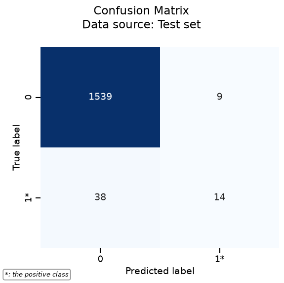
Accuracy can be inflated by nearly always predicting the majority class. F1 averages precision and recall into one number and hides which side of the trade-off you care about, so we do not use it here. At the default probability cut-off of 0.5, minority recall is often weak because rare events receive small predicted probabilities.
report.metrics.summarize(
    metric=["accuracy", "precision", "recall", "roc_auc", "log_loss"],
    data_source="both",
).frame()
The stratified hold-out still has only a few dozen type-5 rows against about 1,500 majority rows. Most of those scarce positives are predicted as majority, so minority recall is low while accuracy stays high.
report.metrics.confusion_matrix().plot()
<Figure size 600x600 with 1 Axes>
Check ranking and calibration first#
Before touching thresholds, ask whether probabilities are any good:
ROC AUC asks whether positives tend to get higher scores than negatives (threshold-free ranking),
log-loss penalizes confident wrong probabilities,
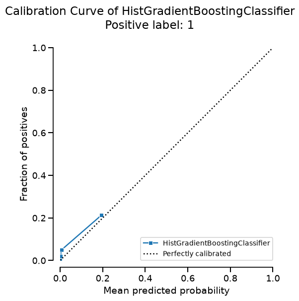
a calibration curve asks whether predicted probabilities match observed frequencies.
On the calibration plot, bins of predicted probability are compared to the fraction of true positives in each bin. A useful curve hugs the diagonal: when the model says “20 %”, about 20 % of those rows really are positive. Points above the diagonal mean under-confidence (events happen more often than predicted); points below mean over-confidence (the model is too sure). With a rare class, almost all mass sits at low probabilities, so the curve often only appears on the left of the plot; that is expected, not a plotting bug.
If ranking and calibration look reasonable, the model may already be useful;
the default 0.5 cut-off is simply the wrong operating point for a rare class.
The next section shows how class_weight="balanced" can push the curve
below the diagonal by inflating minority probabilities.
report.metrics.summarize(
    metric=["roc_auc", "log_loss"],
    data_source="test",
).frame()
metric
roc_auc     0.909586
log_loss    0.112095
Name: HistGradientBoostingClassifier, dtype: float64
report.inspection.calibration_curve(data_source="test", n_bins=10).plot()
<Figure size 600x600 with 1 Axes>
Class weights as a cautionary comparison#
A common reflex is class_weight="balanced". Rebalancing with weights is
equivalent in spirit to resampling methods such as SMOTE or random
oversampling / undersampling: they change the effective class mix and will
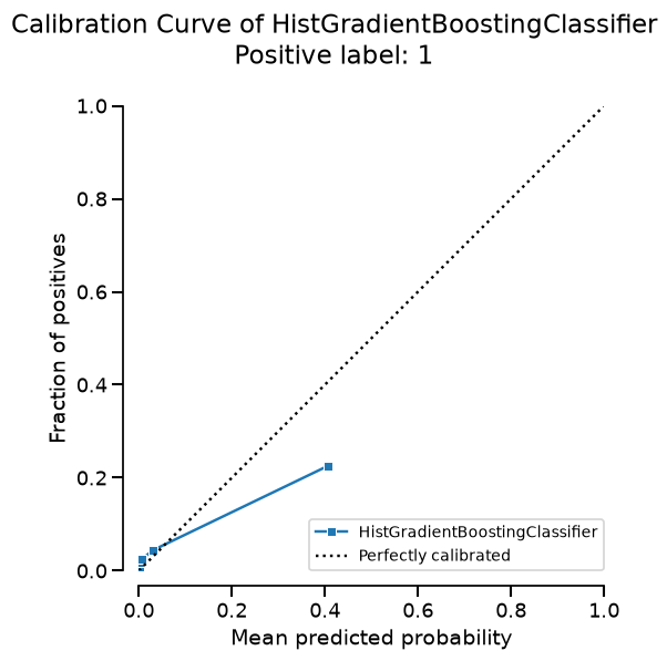
suffer from the same issues. That often improves precision / recall at 0.5
because it inflates minority probabilities, but it typically breaks
calibration: predicted probabilities run ahead of observed rates, so the
curve drifts below the diagonal (over-confidence on the originally rare
class). If you later recalibrate, the thresholded gains often disappear. We
show the comparison, then leave weights behind when calibrated probabilities
matter.
from skore import compare

report_weighted = evaluate(
    HistGradientBoostingClassifier(class_weight="balanced", random_state=42),
    X=X,
    y=y,
    pos_label=1,
    splitter=splitter,
)

comparison_weights = compare(
    {"default": report, "class_weight_balanced": report_weighted}
)
comparison_weights.metrics.summarize(
    metric=["precision", "recall", "roc_auc", "log_loss"],
    data_source="test",
).frame()
After reweighting, compare this curve to the default one: points tend to sit further below the diagonal (over-confident on the rare class).
report_weighted.inspection.calibration_curve(data_source="test", n_bins=10).plot()
<Figure size 600x600 with 1 Axes>
Tune the decision threshold#
Keep the default, prevalence-correct model and change only the decision rule. For this demo we require at least 30 % precision on type 5, then maximize recall. That floor is an explicit product choice: high enough to limit false alarms, low enough that a rare-event model can still catch a useful share of true type-5 stands. Replace 0.3 with a cost or capacity constraint in real work.
TunedThresholdClassifierCV searches the
cut-off by cross-validation and does not change predict_proba, so
calibration stays intact.
from sklearn.metrics import make_scorer, precision_score, recall_score
from sklearn.model_selection import TunedThresholdClassifierCV


def recall_with_min_precision(y_true, y_pred, precision_level=0.3):
    """Maximize recall only among thresholds that keep precision high enough."""
    precision = precision_score(y_true, y_pred, zero_division=0)
    recall = recall_score(y_true, y_pred, zero_division=0)
    if precision < precision_level:
        return -np.inf
    return recall


threshold_scoring = make_scorer(recall_with_min_precision, precision_level=0.3)

tuned = TunedThresholdClassifierCV(
    estimator=HistGradientBoostingClassifier(random_state=42),
    scoring=threshold_scoring,
    cv=3,
    n_jobs=4,
)

report_tuned = evaluate(
    tuned,
    X=X,
    y=y,
    pos_label=1,
    splitter=splitter,
)
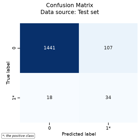
SKD004 still fires: label counts did not change. That is expected. We improved how we decide, not the histogram SKD004 reads. Ignore SKD008 to avoid correlated-feature warnings from Covertype’s constant soil one-hots.
report_tuned.checks.summarize(fast_mode=True, ignore=["SKD008"])
print("Chosen decision threshold:", float(report_tuned.estimator_.best_threshold_))

report_tuned.metrics.summarize(
    metric=["accuracy", "precision", "recall", "roc_auc", "log_loss"],
    data_source="both",
).frame()
Chosen decision threshold: 0.020068079655242547
report_tuned.metrics.confusion_matrix().plot()
<Figure size 600x600 with 1 Axes>
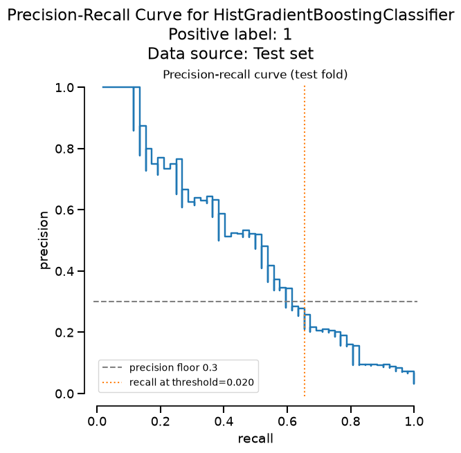
Compare the default 0.5 cut-off to the tuned threshold. Same underlying probabilities; only the hard predictions change. Precision / recall move; ROC AUC and log-loss stay essentially the same.
The scorer asks for precision of at least 0.3, then maximizes recall: catch more type-5 stands without too many false alarms (fraud review, maintenance tickets, medical triage). Preferring high precision instead fits cases where a false alarm is costly: auto-blocking users, expensive tests, or limited outreach budgets.
comparison_thresholds = compare(
    {
        "default_threshold_0.5": report,
        "tuned_threshold": report_tuned,
    }
)
comparison_thresholds.metrics.summarize(
    metric=["precision", "recall", "roc_auc", "log_loss"],
    data_source="test",
).frame()
Inspect the precision-recall curve#
The dashed line is our precision floor (0.3). The tuned threshold should land near the highest-recall point that still respects that floor.
threshold = float(report_tuned.estimator_.best_threshold_)

display = report.metrics.precision_recall()
fig = display.plot()
ax = fig.axes[0]
ax.axhline(0.3, linestyle="--", color="gray", label="precision floor 0.3")
ax.axvline(
    report_tuned.metrics.recall(),
    linestyle=":",
    color="C1",
    label=f"recall at threshold={threshold:.3f}",
)
ax.legend(loc="best")
ax.set_title("Precision-recall curve (test fold)")
fig
<Figure size 600x725 with 1 Axes>
Collecting more minority data#
Gathering more type-5 plots can help the model see the rare class. If acquisition preferentially samples minority rows, train prevalence no longer matches production. Probabilities and thresholds fitted on that mix will be biased unless you correct for the shift. Clearing SKD004 by stuffing minority rows into the table is therefore not automatically a success.
Conclusion#
SKD004 warns that one class dominates the table. Keep natural prevalence when you need honest probabilities; move the threshold when you need a different precision / recall trade-off. Class weights and resampling are risky shortcuts if calibration matters for the decisions you deploy.
Total running time of the script: (1 minutes 24.225 seconds)