Hub skore Project

This example shows how to use Project in hub mode: store reports remotely and inspect them. A key point is that summarize() returns a Summary, which is a pandas.DataFrame. In Jupyter you get an interactive widget, but you can always inspect and filter the summary as a DataFrame if you prefer.

Examples

To run this example and push in your own Skore Hub workspace and project, you can run this example with the following command:

WORKSPACE=<workspace> PROJECT=<project> python plot_skore_hub_project.py

In this gallery, we are going to push the different reports into a public workspace.

from skore import login

login()

╭───────────────────────────────── Login to Skore Hub ─────────────────────────────────╮
│                                                                                      │
│                        Successfully logged in, using API key.                        │
│                                                                                      │
╰──────────────────────────────────────────────────────────────────────────────────────╯

from sklearn.datasets import load_breast_cancer
from sklearn.linear_model import LogisticRegression
from skore import train_test_split
from skrub import tabular_pipeline

X, y = load_breast_cancer(return_X_y=True, as_frame=True)
split_data = train_test_split(X=X, y=y, random_state=42, as_dict=True)
estimator = tabular_pipeline(LogisticRegression(max_iter=1_000))

╭────────────────────── HighClassImbalanceTooFewExamplesWarning ───────────────────────╮
│ It seems that you have a classification problem with at least one class with fewer   │
│ than 100 examples in the test set. In this case, using train_test_split may not be a │
│ good idea because of high variability in the scores obtained on the test set. We     │
│ suggest three options to tackle this challenge: you can increase test_size, collect  │
│ more data, or use skore's CrossValidationReport with the `splitter` parameter of     │
│ your choice.                                                                         │
╰──────────────────────────────────────────────────────────────────────────────────────╯
╭───────────────────────────────── ShuffleTrueWarning ─────────────────────────────────╮
│ We detected that the `shuffle` parameter is set to `True` either explicitly or from  │
│ its default value. In case of time-ordered events (even if they are independent),    │
│ this will result in inflated model performance evaluation because natural drift will │
│ not be taken into account. We recommend setting the shuffle parameter to `False` in  │
│ order to ensure the evaluation process is really representative of your production   │
│ release process.                                                                     │
╰──────────────────────────────────────────────────────────────────────────────────────╯

from numpy import logspace
from sklearn.base import clone
from skore import EstimatorReport, Project

project = Project(f"{WORKSPACE}/{PROJECT}", mode="hub")

for regularization in logspace(-3, 3, 5):
    project.put(
        f"lr-regularization-{regularization:.1e}",
        EstimatorReport(
            clone(estimator).set_params(logisticregression__C=regularization),
            **split_data,
            pos_label=1,
        ),
    )

  Putting lr-regularization-1.0e-03 0:00:32
Consult your report at
https://skore.probabl.ai/skore/example-skore-hub-project-dev/estimators/1414


  Putting lr-regularization-3.2e-02 0:00:29
Consult your report at
https://skore.probabl.ai/skore/example-skore-hub-project-dev/estimators/1415


  Putting lr-regularization-1.0e+00 0:00:30
Consult your report at
https://skore.probabl.ai/skore/example-skore-hub-project-dev/estimators/1416


  Putting lr-regularization-3.2e+01 0:00:27
Consult your report at
https://skore.probabl.ai/skore/example-skore-hub-project-dev/estimators/1417


  Putting lr-regularization-1.0e+03 0:00:28
Consult your report at
https://skore.probabl.ai/skore/example-skore-hub-project-dev/estimators/1418

Summarize: you get a DataFrame

summarize() returns a Summary, which subclasses pandas.DataFrame. In a Jupyter environment it renders an interactive parallel-coordinates widget by default.

summary = project.summarize()

To see the normal DataFrame table instead of the widget (e.g. in scripts or when you prefer the table), wrap the summary in pandas.DataFrame:

import pandas as pd

pandas_summary = pd.DataFrame(summary)
pandas_summary

		key	date	learner	ml_task	report_type	dataset	rmse	log_loss	roc_auc	fit_time	predict_time	rmse_mean	log_loss_mean	roc_auc_mean	fit_time_mean	predict_time_mean
	id
0	skore:report:estimator:1414	lr-regularization-1.0e-03	2026-03-12T17:00:17.651281+00:00	LogisticRegression	binary-classification	estimator	0966e6e4b6a8c8bd5b0e6bd95f36939d	None	0.388992	0.995214	0.102765	0.086550	None	None	None	None	None
1	skore:report:estimator:1415	lr-regularization-3.2e-02	2026-03-12T17:00:47.335332+00:00	LogisticRegression	binary-classification	estimator	0966e6e4b6a8c8bd5b0e6bd95f36939d	None	0.114416	0.998752	0.278121	0.048624	None	None	None	None	None
2	skore:report:estimator:1416	lr-regularization-1.0e+00	2026-03-12T17:01:17.493650+00:00	LogisticRegression	binary-classification	estimator	0966e6e4b6a8c8bd5b0e6bd95f36939d	None	0.054072	0.997919	0.083589	0.047763	None	None	None	None	None
3	skore:report:estimator:1417	lr-regularization-3.2e+01	2026-03-12T17:01:45.585105+00:00	LogisticRegression	binary-classification	estimator	0966e6e4b6a8c8bd5b0e6bd95f36939d	None	0.084849	0.996255	0.074548	0.039840	None	None	None	None	None
4	skore:report:estimator:1418	lr-regularization-1.0e+03	2026-03-12T17:02:14.218454+00:00	LogisticRegression	binary-classification	estimator	0966e6e4b6a8c8bd5b0e6bd95f36939d	None	0.584540	0.988140	0.076501	0.038711	None	None	None	None	None

Basically, our summary contains metadata related to various information that we need to quickly help filtering the reports.

summary.info()

<class 'skore._project._summary.Summary'>
MultiIndex: 5 entries, (0, 'skore:report:estimator:1414') to (4, 'skore:report:estimator:1418')
Data columns (total 16 columns):
 #   Column             Non-Null Count  Dtype
---  ------             --------------  -----
 0   key                5 non-null      object
 1   date               5 non-null      object
 2   learner            5 non-null      category
 3   ml_task            5 non-null      object
 4   report_type        5 non-null      object
 5   dataset            5 non-null      object
 6   rmse               0 non-null      object
 7   log_loss           5 non-null      float64
 8   roc_auc            5 non-null      float64
 9   fit_time           5 non-null      float64
 10  predict_time       5 non-null      float64
 11  rmse_mean          0 non-null      object
 12  log_loss_mean      0 non-null      object
 13  roc_auc_mean       0 non-null      object
 14  fit_time_mean      0 non-null      object
 15  predict_time_mean  0 non-null      object
dtypes: category(1), float64(4), object(11)
memory usage: 1.1+ KB

Filter reports by metric (e.g. keep only those above a given accuracy) and work with the result as a table.

summary.query("log_loss < 0.1")["key"].tolist()

['lr-regularization-1.0e+00', 'lr-regularization-3.2e+01']

Use reports() to load the corresponding reports from the project (optionally after filtering the summary).

reports = summary.query("log_loss < 0.1").reports(return_as="comparison")
len(reports.reports_)

2

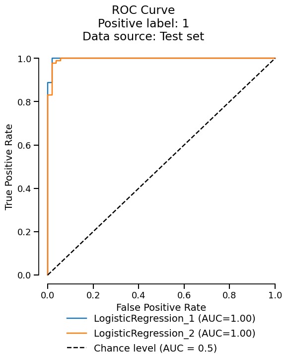
Since we got a ComparisonReport, we can use the metrics accessor to summarize the metrics across the reports.

reports.metrics.summarize().frame()

Estimator	LogisticRegression_1	LogisticRegression_2
Metric
Accuracy	0.993007	0.965035
Precision	0.988889	0.988372
Recall	1.000000	0.955056
ROC AUC	0.997919	0.996255
Brier score	0.013810	0.023881
Fit time (s)	0.083589	0.074548
Predict time (s)	0.039316	0.038926

reports.metrics.roc().plot(subplot_by=None)