SKD008 - Highly correlated input features

This example walks through mitigations when check SKD008 fires because numeric columns are nearly redundant. The check computes pairwise Spearman correlation on training inputs and flags pairs with \(|ρ| > 0.9\).

We showcase the following mitigations from the Automated checks user guide:

• remove or combine redundant features,

• use L1/L2 regularization models as Ridge or Lasso in regression or a penalized LogisticRegression,

• group correlated features before inspecting importance.

We use the breast cancer Wisconsin dataset, where radius, perimeter, and area measurements are almost linearly related. The goal is to simplify the feature table without losing signal.

Load the breast cancer Wisconsin dataset

The dataset describes cell nuclei with 30 numeric features pertaining to cell size, shape, and texture. Many of these features are correlated; the check should help detect this. Class 0 is malignant (our positive label of interest).

from sklearn.datasets import load_breast_cancer

X, y = load_breast_cancer(as_frame=True, return_X_y=True)
pos_label = 0  # malignant

The target is moderately imbalanced but easy to separate; anyway, our concern in this example is collinearity of features.

from skrub import TableReport

TableReport(y)

Please enable javascript

The skrub table reports need javascript to display correctly. If you are displaying a report in a Jupyter notebook and you see this message, you may need to re-execute the cell or to trust the notebook (button on the top right or "File > Trust notebook").

Let us use a stratified TrainTestSplit so both classes appear in train and test.

from skore import TrainTestSplit

splitter = TrainTestSplit(random_state=42, stratify=y)

Trigger SKD008: full feature set

A gradient boosting classifier tolerates correlated inputs, but SKD008 still inspects the training matrix. Let us fit on the full table, then summarize checks.

from sklearn.ensemble import HistGradientBoostingClassifier
from skore import evaluate

report = evaluate(
    HistGradientBoostingClassifier(random_state=42),
    X=X,
    y=y,
    splitter=splitter,
    pos_label=pos_label,
)

SKD008 gives the number of highly correlated feature pairs on the training fold.

report.checks.summarize(fast_mode=True)

Investigate correlated pairs

The check prompts us to look more closely at the data. The TableReport “Associations” tab indeed shows many highly correlated feature pairs (for instance radius, perimeter, and area within each size block).

TableReport(X)

Please enable javascript

The skrub table reports need javascript to display correctly. If you are displaying a report in a Jupyter notebook and you see this message, you may need to re-execute the cell or to trust the notebook (button on the top right or "File > Trust notebook").

Remove redundant features

One way to satisfy the check is to drop some of the correlated features. Let us drop:

• perimeter and area within each size block since they are correlated with radius,

• the “error” and “worst” features,

• the features highly correlated with mean concavity.

We put the drop inside a FunctionTransformer so the same column selection is applied on train and test as part of the estimator.

from sklearn.pipeline import make_pipeline
from sklearn.preprocessing import FunctionTransformer

cols_to_drop = [
    "mean perimeter",
    "mean area",
    "mean concave points",
    "mean compactness",
] + [c for c in X.columns if "worst" in c or "error" in c]


def drop_redundant_features(X_df):
    return X_df.drop(columns=[c for c in cols_to_drop if c in X_df.columns])


model_dropped = make_pipeline(
    FunctionTransformer(drop_redundant_features),
    HistGradientBoostingClassifier(random_state=42),
)

report_dropped = evaluate(
    model_dropped,
    X=X,
    y=y,
    splitter=splitter,
    pos_label=pos_label,
)

SKD008 no longer fires.

report_dropped.checks.summarize(fast_mode=True)

Group correlated features by clustering

Rather than hand-picking groups and averaging them, we follow the same idea as the scikit-learn example on permutation importance with multicollinear features: hierarchical clustering on Spearman correlations, then keep one feature per cluster. We build the linkage on the training fold of the full-feature report so the grouping does not peek at the test set.

from collections import defaultdict

import matplotlib.pyplot as plt
import numpy as np
import pandas as pd
from scipy.cluster import hierarchy
from scipy.spatial.distance import squareform
from scipy.stats import spearmanr

X_train = report.X_train
corr = spearmanr(X_train).correlation
corr = (corr + corr.T) / 2
np.fill_diagonal(corr, 1)
distance_matrix = 1 - np.abs(corr)
dist_linkage = hierarchy.ward(squareform(distance_matrix))

fig, ax = plt.subplots(figsize=(10, 4))
hierarchy.dendrogram(
    dist_linkage,
    labels=X_train.columns.to_list(),
    ax=ax,
    leaf_rotation=90,
)
ax.set_title("Hierarchical clustering of features (Spearman distance)")
fig.tight_layout()
_ = fig

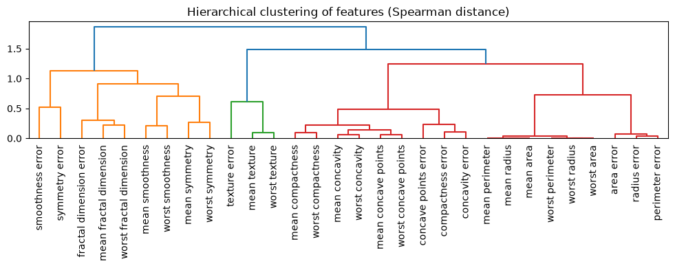
Cutting the dendrogram at distance 1 (as in the scikit-learn example) yields compact clusters. Inspecting them, we recover familiar blocks such as radius / perimeter / area, or the texture triplet — similar to the hand-built groups one might have written from the Associations tab.

cluster_ids = hierarchy.fcluster(dist_linkage, t=1, criterion="distance")
cluster_id_to_features = defaultdict(list)
for feature_name, cluster_id in zip(X_train.columns, cluster_ids, strict=True):
    cluster_id_to_features[int(cluster_id)].append(feature_name)

cluster_table = (
    pd.Series(
        {
            cid: ", ".join(names)
            for cid, names in sorted(cluster_id_to_features.items())
        },
        name="features",
    )
    .rename_axis("cluster")
    .reset_index()
)
cluster_table

	cluster	features
0	1	smoothness error, symmetry error
1	2	mean smoothness, mean symmetry, mean fractal d...
2	3	mean texture, texture error, worst texture
3	4	mean compactness, mean concavity, mean concave...
4	5	mean radius, mean perimeter, mean area, radius...

Keep the first feature of each cluster and wrap that selection in the pipeline.

selected_features = [names[0] for names in cluster_id_to_features.values()]
selected_features


def keep_cluster_representatives(X_df, columns=selected_features):
    return X_df.loc[:, columns]


model_clustered = make_pipeline(
    FunctionTransformer(keep_cluster_representatives),
    HistGradientBoostingClassifier(random_state=42),
)

report_clustered = evaluate(
    model_clustered,
    X=X,
    y=y,
    splitter=splitter,
    pos_label=pos_label,
)

SKD008 no longer fires.

report_clustered.checks.summarize(fast_mode=True)

Compare strategies

compare() contrasts test metrics for the full, dropped, and cluster-selected feature tables on the same stratified split. This dataset is really simple so the metrics are not that different between the three strategies.

from skore import compare

comparison = compare(
    {
        "full_features": report,
        "dropped_redundant": report_dropped,
        "cluster_representatives": report_clustered,
    }
)
comparison.metrics.summarize(data_source="both").frame()

	full_features (train)	full_features (test)	dropped_redundant (train)	dropped_redundant (test)	cluster_representatives (train)	cluster_representatives (test)
metric
accuracy	1.000000	0.956140	1.000000	0.938596	1.000000	0.912281
precision	1.000000	0.974359	1.000000	0.926829	1.000000	0.863636
recall	1.000000	0.904762	1.000000	0.904762	1.000000	0.904762
roc_auc	1.000000	0.990079	1.000000	0.983135	1.000000	0.968254
log_loss	0.000644	0.133771	0.003194	0.189599	0.004918	0.357143
brier_score	0.000003	0.033279	0.000079	0.047430	0.000165	0.083249
fit_time	0.165602	0.165602	0.098327	0.098327	0.162023	0.162023
predict_time	0.004058	0.002134	0.004279	0.002345	0.006327	0.003864

Note: L1 logistic regression does not clear SKD008

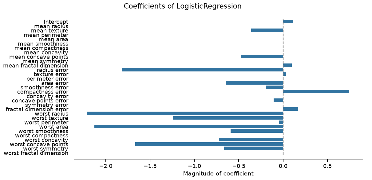
LogisticRegression with an L1 penalty can shrink coefficients of redundant inputs toward zero (a classification analogue of Lasso). SKD008 only inspects the input matrix, so the check still fires; once that is understood, mute it and inspect which features the penalized model kept.

import skore
from sklearn.linear_model import LogisticRegression
from sklearn.preprocessing import StandardScaler

model_l1 = make_pipeline(
    StandardScaler(),
    LogisticRegression(
        l1_ratio=1.0,
        solver="saga",
        max_iter=5_000,
        random_state=42,
    ),
)

report_l1 = evaluate(
    model_l1,
    X=X,
    y=y,
    splitter=splitter,
    pos_label=pos_label,
)

SKD008 still fires on the correlated inputs.

report_l1.checks.summarize(fast_mode=True)

Mute the expected tip and look at the fitted coefficients: many correlated features are driven to zero.

with skore.configuration(ignore_checks=["SKD008"]):
    muted = report_l1.checks.summarize(fast_mode=True)
muted

_ = report_l1.inspection.coefficients().plot()

Conclusion

SKD008 highlights redundant numeric features that may cause the fitting to fail or complicate interpretation. Here, the Associations view and Spearman clustering guided dropping and selecting cluster representatives; L1 LogisticRegression can shrink coefficients but does not clear the check, so mute SKD008 once that behavior is expected. Choose dropping or cluster-based selection based on how you want to modify the feature table.