Note
Go to the end to download the full example code.
Local skore Project#
This example shows how to use Project in local mode: store
reports on your machine and inspect them. A key point is that
summarize() returns a Summary object that holds the
metadata and metrics of every report. In Jupyter it renders as an interactive
table with three views (Table, parallel-coordinates Plot, and Trend) where you
can filter and pick reports to build a query string; the underlying
pandas.DataFrame is accessible through its frame method.
Create a local project and store reports#
We use a temporary directory as the workspace so the example is self-contained.
In practice you can omit workspace to use the default (e.g. a skore/
directory in your user cache).
from pathlib import Path
from tempfile import TemporaryDirectory

from skore import Project

tmp_dir = TemporaryDirectory()
tmp_path = Path(tmp_dir.name)
project = Project("example-project", workspace=tmp_path)
from sklearn.datasets import load_breast_cancer
from sklearn.linear_model import LogisticRegression
from skrub import tabular_pipeline

X, y = load_breast_cancer(return_X_y=True, as_frame=True)
estimator = tabular_pipeline(LogisticRegression(max_iter=1_000))
import numpy as np
from sklearn.base import clone
from skore import evaluate

for regularization in np.logspace(-7, 7, 31):
    report = evaluate(
        clone(estimator).set_params(logisticregression__C=regularization),
        X,
        y,
        splitter=0.2,
        pos_label=1,
    )
    project.put(f"lr-regularization-{regularization:.1e}", report)
Summarize: you get a Summary#
summarize() returns a Summary object. In a
Jupyter environment it renders as an interactive table where you can filter rows and
pick reports across the different views; the selection produces a query string ready
to pass to query().
Filter reports by metric (e.g. keep only those above a given accuracy) and work with the result as a table.
summary.query("log_loss < 0.1")
/home/runner/work/skore/skore/skore/venv/lib/python3.14/site-packages/skore/_project/_summary.py:67: SettingWithCopyWarning:
A value is trying to be set on a copy of a slice from a DataFrame.
Try using .loc[row_indexer,col_indexer] = value instead

See the caveats in the documentation: https://pandas.pydata.org/pandas-docs/stable/user_guide/indexing.html#returning-a-view-versus-a-copy
  dataframe["date"] = to_datetime(dataframe["date"], errors="coerce")
/home/runner/work/skore/skore/skore/venv/lib/python3.14/site-packages/skore/_project/_summary.py:68: SettingWithCopyWarning:
A value is trying to be set on a copy of a slice from a DataFrame.
Try using .loc[row_indexer,col_indexer] = value instead

See the caveats in the documentation: https://pandas.pydata.org/pandas-docs/stable/user_guide/indexing.html#returning-a-view-versus-a-copy
  dataframe["learner"] = Categorical(dataframe["learner"])
/home/runner/work/skore/skore/skore/venv/lib/python3.14/site-packages/skore/_project/_summary.py:70: SettingWithCopyWarning:
A value is trying to be set on a copy of a slice from a DataFrame.
Try using .loc[row_indexer,col_indexer] = value instead

See the caveats in the documentation: https://pandas.pydata.org/pandas-docs/stable/user_guide/indexing.html#returning-a-view-versus-a-copy
  dataframe[column] = dataframe[column].astype("string")
Use compare() to load the corresponding reports from the
project (optionally after filtering the summary). Passing return_as="report"
returns a ComparisonReport built from those reports.
reports = summary.query("log_loss < 0.1").compare(return_as="report")
reports
/home/runner/work/skore/skore/skore/venv/lib/python3.14/site-packages/skore/_project/_summary.py:67: SettingWithCopyWarning:
A value is trying to be set on a copy of a slice from a DataFrame.
Try using .loc[row_indexer,col_indexer] = value instead

See the caveats in the documentation: https://pandas.pydata.org/pandas-docs/stable/user_guide/indexing.html#returning-a-view-versus-a-copy
  dataframe["date"] = to_datetime(dataframe["date"], errors="coerce")
/home/runner/work/skore/skore/skore/venv/lib/python3.14/site-packages/skore/_project/_summary.py:68: SettingWithCopyWarning:
A value is trying to be set on a copy of a slice from a DataFrame.
Try using .loc[row_indexer,col_indexer] = value instead

See the caveats in the documentation: https://pandas.pydata.org/pandas-docs/stable/user_guide/indexing.html#returning-a-view-versus-a-copy
  dataframe["learner"] = Categorical(dataframe["learner"])
/home/runner/work/skore/skore/skore/venv/lib/python3.14/site-packages/skore/_project/_summary.py:70: SettingWithCopyWarning:
A value is trying to be set on a copy of a slice from a DataFrame.
Try using .loc[row_indexer,col_indexer] = value instead

See the caveats in the documentation: https://pandas.pydata.org/pandas-docs/stable/user_guide/indexing.html#returning-a-view-versus-a-copy
  dataframe[column] = dataframe[column].astype("string")
/home/runner/work/skore/skore/skore/venv/lib/python3.14/site-packages/skore/_project/_summary.py:70: SettingWithCopyWarning:
A value is trying to be set on a copy of a slice from a DataFrame.
Try using .loc[row_indexer,col_indexer] = value instead

See the caveats in the documentation: https://pandas.pydata.org/pandas-docs/stable/user_guide/indexing.html#returning-a-view-versus-a-copy
  dataframe[column] = dataframe[column].astype("string")
/home/runner/work/skore/skore/skore/venv/lib/python3.14/site-packages/skore/_project/_summary.py:70: SettingWithCopyWarning:
A value is trying to be set on a copy of a slice from a DataFrame.
Try using .loc[row_indexer,col_indexer] = value instead

See the caveats in the documentation: https://pandas.pydata.org/pandas-docs/stable/user_guide/indexing.html#returning-a-view-versus-a-copy
  dataframe[column] = dataframe[column].astype("string")
/home/runner/work/skore/skore/skore/venv/lib/python3.14/site-packages/skore/_project/_summary.py:70: SettingWithCopyWarning:
A value is trying to be set on a copy of a slice from a DataFrame.
Try using .loc[row_indexer,col_indexer] = value instead

See the caveats in the documentation: https://pandas.pydata.org/pandas-docs/stable/user_guide/indexing.html#returning-a-view-versus-a-copy
  dataframe[column] = dataframe[column].astype("string")
| Metric | LogisticRegression_1 | LogisticRegression_2 | LogisticRegression_3 | LogisticRegression_4 |
|---|---|---|---|---|
| Score | 0.947368 | 0.964912 | 0.964912 | 0.964912 |
| Accuracy | 0.947368 | 0.964912 | 0.964912 | 0.964912 |
| Precision | 0.942029 | 0.970149 | 0.970149 | 0.970149 |
| Recall | 0.970149 | 0.970149 | 0.970149 | 0.970149 |
| ROC AUC | 0.996189 | 0.995872 | 0.995554 | 0.994601 |
| Log loss | 0.098897 | 0.083941 | 0.080457 | 0.089466 |
| Brier score | 0.027157 | 0.024990 | 0.025149 | 0.026218 |
| Fit time (s) | 0.117023 | 0.111087 | 0.111584 | 0.114038 |
| Predict time (s) | 0.069400 | 0.070784 | 0.071434 | 0.065870 |
Pipeline(steps=[('tablevectorizer',
                 TableVectorizer(datetime=DatetimeEncoder(periodic_encoding='spline'))),
                ('simpleimputer', SimpleImputer(add_indicator=True)),
                ('squashingscaler', SquashingScaler(max_absolute_value=5)),
                ('logisticregression',
                 LogisticRegression(C=np.float64(0.11659144011798311),
                                    max_iter=1000))])
In a Jupyter environment, please rerun this cell to show the HTML representation or trust the notebook. On GitHub, the HTML representation is unable to render, please try loading this page with nbviewer.org.
Parameters
Fitted attributes
Parameters
| low_cardinality | OneHotEncoder..._output=False) | |
| high_cardinality | StringEncoder() | |
| numeric | PassThrough() | |
| datetime | DatetimeEncod...ding='spline') | |
| cardinality_threshold | 40 | |
| specific_transformers | () | |
| drop_null_fraction | 1.0 | |
| drop_if_constant | False | |
| drop_if_unique | False | |
| datetime_format | None | |
| null_strings | None | |
| n_jobs | None |
Fitted attributes
| Name | Type | Value |
|---|---|---|
| all_outputs_ | list | ['me...us', 'me...re', 'me...er', 'me...ea', ...] |
| all_processing_steps_ | dict | {'ar...or': [DropUninformative(), ToFloat(), PassThrough(), {'area error': ToFloat()}], 'co...or': [DropUninformative(), ToFloat(), PassThrough(), {'compactness...r': ToFloat()}], 'co...or': [DropUninformative(), ToFloat(), PassThrough(), {'concave poi...r': ToFloat()}], 'co...or': [DropUninformative(), ToFloat(), PassThrough(), {'concavity error': ToFloat()}], ...} |
| column_to_kind_ | dict | {'ar...or': 'numeric', 'co...or': 'numeric', 'co...or': 'numeric', 'co...or': 'numeric', ...} |
| feature_names_in_ | list | ['me...us', 'me...re', 'me...er', 'me...ea', ...] |
| input_to_outputs_ | dict | {'ar...or': ['ar...or'], 'co...or': ['co...or'], 'co...or': ['co...or'], 'co...or': ['co...or'], ...} |
| kind_to_columns_ | dict | {'da...me': [], 'hi...ty': [], 'lo...ty': [], 'numeric': ['me...us', 'me...re', 'me...er', 'me...ea', ...], ...} |
| n_features_in_ | int | 30 |
| output_to_input_ | dict | {'ar...or': 'ar...or', 'co...or': 'co...or', 'co...or': 'co...or', 'co...or': 'co...or', ...} |
| transformers_ | dict | {'ar...or': PassThrough(), 'co...or': PassThrough(), 'co...or': PassThrough(), 'co...or': PassThrough(), ...} |
['mean radius', 'mean texture', 'mean perimeter', 'mean area', 'mean smoothness', 'mean compactness', 'mean concavity', 'mean concave points', 'mean symmetry', 'mean fractal dimension', 'radius error', 'texture error', 'perimeter error', 'area error', 'smoothness error', 'compactness error', 'concavity error', 'concave points error', 'symmetry error', 'fractal dimension error', 'worst radius', 'worst texture', 'worst perimeter', 'worst area', 'worst smoothness', 'worst compactness', 'worst concavity', 'worst concave points', 'worst symmetry', 'worst fractal dimension']
Parameters
Parameters
| periodic_encoding | 'spline' | |
| resolution | 'hour' | |
| add_weekday | False | |
| add_total_seconds | True | |
| add_day_of_year | False |
Parameters
Parameters
| n_components | 30 | |
| vectorizer | 'tfidf' | |
| ngram_range | (3, ...) | |
| analyzer | 'char_wb' | |
| stop_words | None | |
| random_state | None | |
| vocabulary | None |
30 features
| mean radius |
| mean texture |
| mean perimeter |
| mean area |
| mean smoothness |
| mean compactness |
| mean concavity |
| mean concave points |
| mean symmetry |
| mean fractal dimension |
| radius error |
| texture error |
| perimeter error |
| area error |
| smoothness error |
| compactness error |
| concavity error |
| concave points error |
| symmetry error |
| fractal dimension error |
| worst radius |
| worst texture |
| worst perimeter |
| worst area |
| worst smoothness |
| worst compactness |
| worst concavity |
| worst concave points |
| worst symmetry |
| worst fractal dimension |
Parameters
Fitted attributes
| Name | Type | Value |
|---|---|---|
|
feature_names_in_
feature_names_in_: ndarray of shape (`n_features_in_`,) Names of features seen during :term:`fit`. Defined only when `X` has feature names that are all strings. .. versionadded:: 1.0 |
ndarray[object](30,) | ['mean radius','mean texture','mean perimeter',...,'worst concave points', 'worst symmetry','worst fractal dimension'] |
|
indicator_
indicator_: :class:`~sklearn.impute.MissingIndicator` Indicator used to add binary indicators for missing values. `None` if `add_indicator=False`. |
MissingIndicator | MissingIndica..._on_new=False) |
|
n_features_in_
n_features_in_: int Number of features seen during :term:`fit`. .. versionadded:: 0.24 |
int | 30 |
|
statistics_
statistics_: array of shape (n_features,) The imputation fill value for each feature. Computing statistics can result in `np.nan` values. During :meth:`transform`, features corresponding to `np.nan` statistics will be discarded. |
ndarray[float64](30,) | [14.11,19.15,91.82,..., 0.11, 0.29, 0.08] |
30 features
| mean radius |
| mean texture |
| mean perimeter |
| mean area |
| mean smoothness |
| mean compactness |
| mean concavity |
| mean concave points |
| mean symmetry |
| mean fractal dimension |
| radius error |
| texture error |
| perimeter error |
| area error |
| smoothness error |
| compactness error |
| concavity error |
| concave points error |
| symmetry error |
| fractal dimension error |
| worst radius |
| worst texture |
| worst perimeter |
| worst area |
| worst smoothness |
| worst compactness |
| worst concavity |
| worst concave points |
| worst symmetry |
| worst fractal dimension |
Parameters
| max_absolute_value | 5 | |
| quantile_range | (25.0, ...) |
Fitted attributes
| Name | Type | Value |
|---|---|---|
| minmax_cols_ | ndarray[bool](30,) | [False,False,False,...,False,False,False] |
| minmax_scaler_ | NoneType | None |
| n_features_in_ | int | 30 |
| robust_cols_ | ndarray[bool](30,) | [ True, True, True,..., True, True, True] |
| robust_scaler_ | RobustScaler | RobustScaler() |
| zero_cols_ | ndarray[bool](30,) | [False,False,False,...,False,False,False] |
30 features
| x0 |
| x1 |
| x2 |
| x3 |
| x4 |
| x5 |
| x6 |
| x7 |
| x8 |
| x9 |
| x10 |
| x11 |
| x12 |
| x13 |
| x14 |
| x15 |
| x16 |
| x17 |
| x18 |
| x19 |
| x20 |
| x21 |
| x22 |
| x23 |
| x24 |
| x25 |
| x26 |
| x27 |
| x28 |
| x29 |
Parameters
Fitted attributes
| mean radius | mean texture | mean perimeter | mean area | mean smoothness | mean compactness | mean concavity | mean concave points | mean symmetry | mean fractal dimension | radius error | texture error | perimeter error | area error | smoothness error | compactness error | concavity error | concave points error | symmetry error | fractal dimension error | worst radius | worst texture | worst perimeter | worst area | worst smoothness | worst compactness | worst concavity | worst concave points | worst symmetry | worst fractal dimension | target | |
|---|---|---|---|---|---|---|---|---|---|---|---|---|---|---|---|---|---|---|---|---|---|---|---|---|---|---|---|---|---|---|---|
| 0 | 10.1 | 17.5 | 64.4 | 311. | 0.101 | 0.0733 | 0.0251 | 0.0177 | 0.189 | 0.0633 | 0.262 | 2.02 | 1.78 | 16.9 | 0.00780 | 0.0145 | 0.0169 | 0.00804 | 0.0210 | 0.00278 | 11.2 | 26.8 | 72.0 | 384. | 0.140 | 0.140 | 0.105 | 0.0650 | 0.289 | 0.0766 | 1 |
| 1 | 10.8 | 22.0 | 68.8 | 360. | 0.0880 | 0.0574 | 0.0361 | 0.0140 | 0.202 | 0.0598 | 0.308 | 1.62 | 2.24 | 20.2 | 0.00654 | 0.0215 | 0.0299 | 0.0104 | 0.0184 | 0.00269 | 12.8 | 32.0 | 83.7 | 490. | 0.130 | 0.170 | 0.193 | 0.0748 | 0.296 | 0.0766 | 1 |
| 2 | 16.1 | 14.9 | 104. | 800. | 0.0950 | 0.0850 | 0.0550 | 0.0453 | 0.173 | 0.0587 | 0.239 | 0.637 | 1.73 | 21.8 | 0.00396 | 0.0125 | 0.0183 | 0.00875 | 0.0150 | 0.00162 | 17.7 | 19.6 | 116. | 948. | 0.121 | 0.172 | 0.231 | 0.113 | 0.278 | 0.0701 | 1 |
| 3 | 12.2 | 17.8 | 77.8 | 451. | 0.104 | 0.0706 | 0.0249 | 0.0294 | 0.190 | 0.0664 | 0.366 | 1.51 | 2.41 | 24.4 | 0.00543 | 0.0118 | 0.0113 | 0.0152 | 0.0222 | 0.00341 | 12.8 | 20.9 | 82.1 | 495. | 0.114 | 0.0936 | 0.0498 | 0.0588 | 0.223 | 0.0738 | 1 |
| 4 | 12.2 | 22.4 | 78.2 | 466. | 0.0819 | 0.0520 | 0.0171 | 0.0126 | 0.154 | 0.0598 | 0.224 | 1.14 | 1.58 | 18.0 | 0.00510 | 0.0120 | 0.00941 | 0.00455 | 0.0161 | 0.00240 | 14.2 | 32.0 | 92.7 | 623. | 0.126 | 0.180 | 0.123 | 0.0634 | 0.310 | 0.0820 | 1 |
| 564 | 17.4 | 25.6 | 114. | 948. | 0.101 | 0.115 | 0.168 | 0.0660 | 0.131 | 0.0587 | 0.530 | 1.67 | 3.77 | 58.5 | 0.0311 | 0.0856 | 0.144 | 0.0393 | 0.0217 | 0.0126 | 18.1 | 28.1 | 120. | 1.02e+03 | 0.124 | 0.179 | 0.280 | 0.110 | 0.160 | 0.0682 | 0 |
| 565 | 12.8 | 16.7 | 82.5 | 494. | 0.113 | 0.112 | 0.0388 | 0.0300 | 0.212 | 0.0662 | 0.383 | 1.00 | 2.50 | 28.6 | 0.00751 | 0.0156 | 0.0198 | 0.00920 | 0.0181 | 0.00363 | 14.4 | 21.7 | 93.6 | 624. | 0.147 | 0.198 | 0.142 | 0.0804 | 0.307 | 0.0856 | 1 |
| 566 | 20.2 | 19.5 | 134. | 1.25e+03 | 0.113 | 0.149 | 0.213 | 0.126 | 0.172 | 0.0605 | 0.433 | 1.00 | 3.01 | 52.5 | 0.00909 | 0.0272 | 0.0555 | 0.0191 | 0.0245 | 0.00400 | 22.0 | 25.1 | 146. | 1.48e+03 | 0.167 | 0.294 | 0.531 | 0.217 | 0.303 | 0.0808 | 0 |
| 567 | 18.3 | 20.6 | 121. | 1.05e+03 | 0.107 | 0.125 | 0.157 | 0.0945 | 0.186 | 0.0594 | 0.545 | 0.922 | 3.22 | 67.4 | 0.00618 | 0.0188 | 0.0291 | 0.0105 | 0.0156 | 0.00272 | 21.9 | 26.2 | 142. | 1.49e+03 | 0.149 | 0.254 | 0.376 | 0.151 | 0.307 | 0.0786 | 0 |
| 568 | 15.0 | 16.7 | 98.7 | 689. | 0.0988 | 0.136 | 0.0772 | 0.0614 | 0.167 | 0.0687 | 0.372 | 0.842 | 2.30 | 34.8 | 0.00412 | 0.0182 | 0.0200 | 0.0100 | 0.0106 | 0.00324 | 16.8 | 20.4 | 110. | 857. | 0.114 | 0.218 | 0.186 | 0.102 | 0.218 | 0.0855 | 1 |
mean radius
Float64DType- Null values
- 0 (0.0%)
- Unique values
-
456 (80.1%)
This column has a high cardinality (> 40).
- Mean ± Std
- 14.1 ± 3.52
- Median ± IQR
- 13.4 ± 4.08
- Min | Max
- 6.98 | 28.1
mean texture
Float64DType- Null values
- 0 (0.0%)
- Unique values
-
479 (84.2%)
This column has a high cardinality (> 40).
- Mean ± Std
- 19.3 ± 4.30
- Median ± IQR
- 18.8 ± 5.63
- Min | Max
- 9.71 | 39.3
mean perimeter
Float64DType- Null values
- 0 (0.0%)
- Unique values
-
522 (91.7%)
This column has a high cardinality (> 40).
- Mean ± Std
- 92.0 ± 24.3
- Median ± IQR
- 86.2 ± 28.9
- Min | Max
- 43.8 | 188.
mean area
Float64DType- Null values
- 0 (0.0%)
- Unique values
-
539 (94.7%)
This column has a high cardinality (> 40).
- Mean ± Std
- 655. ± 352.
- Median ± IQR
- 551. ± 362.
- Min | Max
- 144. | 2.50e+03
mean smoothness
Float64DType- Null values
- 0 (0.0%)
- Unique values
-
474 (83.3%)
This column has a high cardinality (> 40).
- Mean ± Std
- 0.0964 ± 0.0141
- Median ± IQR
- 0.0959 ± 0.0189
- Min | Max
- 0.0526 | 0.163
mean compactness
Float64DType- Null values
- 0 (0.0%)
- Unique values
-
537 (94.4%)
This column has a high cardinality (> 40).
- Mean ± Std
- 0.104 ± 0.0528
- Median ± IQR
- 0.0926 ± 0.0655
- Min | Max
- 0.0194 | 0.345
mean concavity
Float64DType- Null values
- 0 (0.0%)
- Unique values
-
537 (94.4%)
This column has a high cardinality (> 40).
- Mean ± Std
- 0.0888 ± 0.0797
- Median ± IQR
- 0.0615 ± 0.101
- Min | Max
- 0.00 | 0.427
mean concave points
Float64DType- Null values
- 0 (0.0%)
- Unique values
-
542 (95.3%)
This column has a high cardinality (> 40).
- Mean ± Std
- 0.0489 ± 0.0388
- Median ± IQR
- 0.0335 ± 0.0537
- Min | Max
- 0.00 | 0.201
mean symmetry
Float64DType- Null values
- 0 (0.0%)
- Unique values
-
432 (75.9%)
This column has a high cardinality (> 40).
- Mean ± Std
- 0.181 ± 0.0274
- Median ± IQR
- 0.179 ± 0.0338
- Min | Max
- 0.106 | 0.304
mean fractal dimension
Float64DType- Null values
- 0 (0.0%)
- Unique values
-
499 (87.7%)
This column has a high cardinality (> 40).
- Mean ± Std
- 0.0628 ± 0.00706
- Median ± IQR
- 0.0615 ± 0.00842
- Min | Max
- 0.0500 | 0.0974
radius error
Float64DType- Null values
- 0 (0.0%)
- Unique values
-
540 (94.9%)
This column has a high cardinality (> 40).
- Mean ± Std
- 0.405 ± 0.277
- Median ± IQR
- 0.324 ± 0.246
- Min | Max
- 0.112 | 2.87
texture error
Float64DType- Null values
- 0 (0.0%)
- Unique values
-
519 (91.2%)
This column has a high cardinality (> 40).
- Mean ± Std
- 1.22 ± 0.552
- Median ± IQR
- 1.11 ± 0.640
- Min | Max
- 0.360 | 4.88
perimeter error
Float64DType- Null values
- 0 (0.0%)
- Unique values
-
533 (93.7%)
This column has a high cardinality (> 40).
- Mean ± Std
- 2.87 ± 2.02
- Median ± IQR
- 2.29 ± 1.75
- Min | Max
- 0.757 | 22.0
area error
Float64DType- Null values
- 0 (0.0%)
- Unique values
-
528 (92.8%)
This column has a high cardinality (> 40).
- Mean ± Std
- 40.3 ± 45.5
- Median ± IQR
- 24.5 ± 27.3
- Min | Max
- 6.80 | 542.
smoothness error
Float64DType- Null values
- 0 (0.0%)
- Unique values
-
547 (96.1%)
This column has a high cardinality (> 40).
- Mean ± Std
- 0.00704 ± 0.00300
- Median ± IQR
- 0.00638 ± 0.00298
- Min | Max
- 0.00171 | 0.0311
compactness error
Float64DType- Null values
- 0 (0.0%)
- Unique values
-
541 (95.1%)
This column has a high cardinality (> 40).
- Mean ± Std
- 0.0255 ± 0.0179
- Median ± IQR
- 0.0204 ± 0.0194
- Min | Max
- 0.00225 | 0.135
concavity error
Float64DType- Null values
- 0 (0.0%)
- Unique values
-
533 (93.7%)
This column has a high cardinality (> 40).
- Mean ± Std
- 0.0319 ± 0.0302
- Median ± IQR
- 0.0259 ± 0.0270
- Min | Max
- 0.00 | 0.396
concave points error
Float64DType- Null values
- 0 (0.0%)
- Unique values
-
507 (89.1%)
This column has a high cardinality (> 40).
- Mean ± Std
- 0.0118 ± 0.00617
- Median ± IQR
- 0.0109 ± 0.00707
- Min | Max
- 0.00 | 0.0528
symmetry error
Float64DType- Null values
- 0 (0.0%)
- Unique values
-
498 (87.5%)
This column has a high cardinality (> 40).
- Mean ± Std
- 0.0205 ± 0.00827
- Median ± IQR
- 0.0187 ± 0.00832
- Min | Max
- 0.00788 | 0.0790
fractal dimension error
Float64DType- Null values
- 0 (0.0%)
- Unique values
-
545 (95.8%)
This column has a high cardinality (> 40).
- Mean ± Std
- 0.00379 ± 0.00265
- Median ± IQR
- 0.00319 ± 0.00231
- Min | Max
- 0.000895 | 0.0298
worst radius
Float64DType- Null values
- 0 (0.0%)
- Unique values
-
457 (80.3%)
This column has a high cardinality (> 40).
- Mean ± Std
- 16.3 ± 4.83
- Median ± IQR
- 15.0 ± 5.78
- Min | Max
- 7.93 | 36.0
worst texture
Float64DType- Null values
- 0 (0.0%)
- Unique values
-
511 (89.8%)
This column has a high cardinality (> 40).
- Mean ± Std
- 25.7 ± 6.15
- Median ± IQR
- 25.4 ± 8.64
- Min | Max
- 12.0 | 49.5
worst perimeter
Float64DType- Null values
- 0 (0.0%)
- Unique values
-
514 (90.3%)
This column has a high cardinality (> 40).
- Mean ± Std
- 107. ± 33.6
- Median ± IQR
- 97.7 ± 41.3
- Min | Max
- 50.4 | 251.
worst area
Float64DType- Null values
- 0 (0.0%)
- Unique values
-
544 (95.6%)
This column has a high cardinality (> 40).
- Mean ± Std
- 881. ± 569.
- Median ± IQR
- 686. ± 569.
- Min | Max
- 185. | 4.25e+03
worst smoothness
Float64DType- Null values
- 0 (0.0%)
- Unique values
-
411 (72.2%)
This column has a high cardinality (> 40).
- Mean ± Std
- 0.132 ± 0.0228
- Median ± IQR
- 0.131 ± 0.0294
- Min | Max
- 0.0712 | 0.223
worst compactness
Float64DType- Null values
- 0 (0.0%)
- Unique values
-
529 (93.0%)
This column has a high cardinality (> 40).
- Mean ± Std
- 0.254 ± 0.157
- Median ± IQR
- 0.212 ± 0.192
- Min | Max
- 0.0273 | 1.06
worst concavity
Float64DType- Null values
- 0 (0.0%)
- Unique values
-
539 (94.7%)
This column has a high cardinality (> 40).
- Mean ± Std
- 0.272 ± 0.209
- Median ± IQR
- 0.227 ± 0.268
- Min | Max
- 0.00 | 1.25
worst concave points
Float64DType- Null values
- 0 (0.0%)
- Unique values
-
492 (86.5%)
This column has a high cardinality (> 40).
- Mean ± Std
- 0.115 ± 0.0657
- Median ± IQR
- 0.0999 ± 0.0965
- Min | Max
- 0.00 | 0.291
worst symmetry
Float64DType- Null values
- 0 (0.0%)
- Unique values
-
500 (87.9%)
This column has a high cardinality (> 40).
- Mean ± Std
- 0.290 ± 0.0619
- Median ± IQR
- 0.282 ± 0.0675
- Min | Max
- 0.157 | 0.664
worst fractal dimension
Float64DType- Null values
- 0 (0.0%)
- Unique values
-
535 (94.0%)
This column has a high cardinality (> 40).
- Mean ± Std
- 0.0839 ± 0.0181
- Median ± IQR
- 0.0800 ± 0.0206
- Min | Max
- 0.0550 | 0.207
target
Int64DType- Null values
- 0 (0.0%)
- Unique values
- 2 (0.4%)
- Mean ± Std
- 0.627 ± 0.484
- Median ± IQR
- 1 ± 1
- Min | Max
- 0 | 1
No columns match the selected filter: . You can change the column filter in the dropdown menu above.
| Column | Column name | dtype | Is sorted | Null values | Unique values | Mean | Std | Min | Median | Max |
|---|---|---|---|---|---|---|---|---|---|---|
| 0 | mean radius | Float64DType | False | 0 (0.0%) | 456 (80.1%) | 14.1 | 3.52 | 6.98 | 13.4 | 28.1 |
| 1 | mean texture | Float64DType | False | 0 (0.0%) | 479 (84.2%) | 19.3 | 4.30 | 9.71 | 18.8 | 39.3 |
| 2 | mean perimeter | Float64DType | False | 0 (0.0%) | 522 (91.7%) | 92.0 | 24.3 | 43.8 | 86.2 | 188. |
| 3 | mean area | Float64DType | False | 0 (0.0%) | 539 (94.7%) | 655. | 352. | 144. | 551. | 2.50e+03 |
| 4 | mean smoothness | Float64DType | False | 0 (0.0%) | 474 (83.3%) | 0.0964 | 0.0141 | 0.0526 | 0.0959 | 0.163 |
| 5 | mean compactness | Float64DType | False | 0 (0.0%) | 537 (94.4%) | 0.104 | 0.0528 | 0.0194 | 0.0926 | 0.345 |
| 6 | mean concavity | Float64DType | False | 0 (0.0%) | 537 (94.4%) | 0.0888 | 0.0797 | 0.00 | 0.0615 | 0.427 |
| 7 | mean concave points | Float64DType | False | 0 (0.0%) | 542 (95.3%) | 0.0489 | 0.0388 | 0.00 | 0.0335 | 0.201 |
| 8 | mean symmetry | Float64DType | False | 0 (0.0%) | 432 (75.9%) | 0.181 | 0.0274 | 0.106 | 0.179 | 0.304 |
| 9 | mean fractal dimension | Float64DType | False | 0 (0.0%) | 499 (87.7%) | 0.0628 | 0.00706 | 0.0500 | 0.0615 | 0.0974 |
| 10 | radius error | Float64DType | False | 0 (0.0%) | 540 (94.9%) | 0.405 | 0.277 | 0.112 | 0.324 | 2.87 |
| 11 | texture error | Float64DType | False | 0 (0.0%) | 519 (91.2%) | 1.22 | 0.552 | 0.360 | 1.11 | 4.88 |
| 12 | perimeter error | Float64DType | False | 0 (0.0%) | 533 (93.7%) | 2.87 | 2.02 | 0.757 | 2.29 | 22.0 |
| 13 | area error | Float64DType | False | 0 (0.0%) | 528 (92.8%) | 40.3 | 45.5 | 6.80 | 24.5 | 542. |
| 14 | smoothness error | Float64DType | False | 0 (0.0%) | 547 (96.1%) | 0.00704 | 0.00300 | 0.00171 | 0.00638 | 0.0311 |
| 15 | compactness error | Float64DType | False | 0 (0.0%) | 541 (95.1%) | 0.0255 | 0.0179 | 0.00225 | 0.0204 | 0.135 |
| 16 | concavity error | Float64DType | False | 0 (0.0%) | 533 (93.7%) | 0.0319 | 0.0302 | 0.00 | 0.0259 | 0.396 |
| 17 | concave points error | Float64DType | False | 0 (0.0%) | 507 (89.1%) | 0.0118 | 0.00617 | 0.00 | 0.0109 | 0.0528 |
| 18 | symmetry error | Float64DType | False | 0 (0.0%) | 498 (87.5%) | 0.0205 | 0.00827 | 0.00788 | 0.0187 | 0.0790 |
| 19 | fractal dimension error | Float64DType | False | 0 (0.0%) | 545 (95.8%) | 0.00379 | 0.00265 | 0.000895 | 0.00319 | 0.0298 |
| 20 | worst radius | Float64DType | False | 0 (0.0%) | 457 (80.3%) | 16.3 | 4.83 | 7.93 | 15.0 | 36.0 |
| 21 | worst texture | Float64DType | False | 0 (0.0%) | 511 (89.8%) | 25.7 | 6.15 | 12.0 | 25.4 | 49.5 |
| 22 | worst perimeter | Float64DType | False | 0 (0.0%) | 514 (90.3%) | 107. | 33.6 | 50.4 | 97.7 | 251. |
| 23 | worst area | Float64DType | False | 0 (0.0%) | 544 (95.6%) | 881. | 569. | 185. | 686. | 4.25e+03 |
| 24 | worst smoothness | Float64DType | False | 0 (0.0%) | 411 (72.2%) | 0.132 | 0.0228 | 0.0712 | 0.131 | 0.223 |
| 25 | worst compactness | Float64DType | False | 0 (0.0%) | 529 (93.0%) | 0.254 | 0.157 | 0.0273 | 0.212 | 1.06 |
| 26 | worst concavity | Float64DType | False | 0 (0.0%) | 539 (94.7%) | 0.272 | 0.209 | 0.00 | 0.227 | 1.25 |
| 27 | worst concave points | Float64DType | False | 0 (0.0%) | 492 (86.5%) | 0.115 | 0.0657 | 0.00 | 0.0999 | 0.291 |
| 28 | worst symmetry | Float64DType | False | 0 (0.0%) | 500 (87.9%) | 0.290 | 0.0619 | 0.157 | 0.282 | 0.664 |
| 29 | worst fractal dimension | Float64DType | False | 0 (0.0%) | 535 (94.0%) | 0.0839 | 0.0181 | 0.0550 | 0.0800 | 0.207 |
| 30 | target | Int64DType | False | 0 (0.0%) | 2 (0.4%) | 0.627 | 0.484 | 0 | 1 | 1 |
No columns match the selected filter: . You can change the column filter in the dropdown menu above.
Please enable javascript
The skrub table reports need javascript to display correctly. If you are displaying a report in a Jupyter notebook and you see this message, you may need to re-execute the cell or to trust the notebook (button on the top right or "File > Trust notebook").
Pipeline(steps=[('tablevectorizer',
                 TableVectorizer(datetime=DatetimeEncoder(periodic_encoding='spline'))),
                ('simpleimputer', SimpleImputer(add_indicator=True)),
                ('squashingscaler', SquashingScaler(max_absolute_value=5)),
                ('logisticregression',
                 LogisticRegression(C=np.float64(0.34145488738336005),
max_iter=1000))])In a Jupyter environment, please rerun this cell to show the HTML representation or trust the notebook. On GitHub, the HTML representation is unable to render, please try loading this page with nbviewer.org.
Parameters
Fitted attributes
Parameters
| low_cardinality | OneHotEncoder..._output=False) | |
| high_cardinality | StringEncoder() | |
| numeric | PassThrough() | |
| datetime | DatetimeEncod...ding='spline') | |
| cardinality_threshold | 40 | |
| specific_transformers | () | |
| drop_null_fraction | 1.0 | |
| drop_if_constant | False | |
| drop_if_unique | False | |
| datetime_format | None | |
| null_strings | None | |
| n_jobs | None |
Fitted attributes
| Name | Type | Value |
|---|---|---|
| all_outputs_ | list | ['me...us', 'me...re', 'me...er', 'me...ea', ...] |
| all_processing_steps_ | dict | {'ar...or': [DropUninformative(), ToFloat(), PassThrough(), {'area error': ToFloat()}], 'co...or': [DropUninformative(), ToFloat(), PassThrough(), {'compactness...r': ToFloat()}], 'co...or': [DropUninformative(), ToFloat(), PassThrough(), {'concave poi...r': ToFloat()}], 'co...or': [DropUninformative(), ToFloat(), PassThrough(), {'concavity error': ToFloat()}], ...} |
| column_to_kind_ | dict | {'ar...or': 'numeric', 'co...or': 'numeric', 'co...or': 'numeric', 'co...or': 'numeric', ...} |
| feature_names_in_ | list | ['me...us', 'me...re', 'me...er', 'me...ea', ...] |
| input_to_outputs_ | dict | {'ar...or': ['ar...or'], 'co...or': ['co...or'], 'co...or': ['co...or'], 'co...or': ['co...or'], ...} |
| kind_to_columns_ | dict | {'da...me': [], 'hi...ty': [], 'lo...ty': [], 'numeric': ['me...us', 'me...re', 'me...er', 'me...ea', ...], ...} |
| n_features_in_ | int | 30 |
| output_to_input_ | dict | {'ar...or': 'ar...or', 'co...or': 'co...or', 'co...or': 'co...or', 'co...or': 'co...or', ...} |
| transformers_ | dict | {'ar...or': PassThrough(), 'co...or': PassThrough(), 'co...or': PassThrough(), 'co...or': PassThrough(), ...} |
['mean radius', 'mean texture', 'mean perimeter', 'mean area', 'mean smoothness', 'mean compactness', 'mean concavity', 'mean concave points', 'mean symmetry', 'mean fractal dimension', 'radius error', 'texture error', 'perimeter error', 'area error', 'smoothness error', 'compactness error', 'concavity error', 'concave points error', 'symmetry error', 'fractal dimension error', 'worst radius', 'worst texture', 'worst perimeter', 'worst area', 'worst smoothness', 'worst compactness', 'worst concavity', 'worst concave points', 'worst symmetry', 'worst fractal dimension']
Parameters
Parameters
| periodic_encoding | 'spline' | |
| resolution | 'hour' | |
| add_weekday | False | |
| add_total_seconds | True | |
| add_day_of_year | False |
Parameters
Parameters
| n_components | 30 | |
| vectorizer | 'tfidf' | |
| ngram_range | (3, ...) | |
| analyzer | 'char_wb' | |
| stop_words | None | |
| random_state | None | |
| vocabulary | None |
30 features
| mean radius |
| mean texture |
| mean perimeter |
| mean area |
| mean smoothness |
| mean compactness |
| mean concavity |
| mean concave points |
| mean symmetry |
| mean fractal dimension |
| radius error |
| texture error |
| perimeter error |
| area error |
| smoothness error |
| compactness error |
| concavity error |
| concave points error |
| symmetry error |
| fractal dimension error |
| worst radius |
| worst texture |
| worst perimeter |
| worst area |
| worst smoothness |
| worst compactness |
| worst concavity |
| worst concave points |
| worst symmetry |
| worst fractal dimension |
Parameters
Fitted attributes
| Name | Type | Value |
|---|---|---|
|
feature_names_in_
feature_names_in_: ndarray of shape (`n_features_in_`,) Names of features seen during :term:`fit`. Defined only when `X` has feature names that are all strings. .. versionadded:: 1.0 |
ndarray[object](30,) | ['mean radius','mean texture','mean perimeter',...,'worst concave points', 'worst symmetry','worst fractal dimension'] |
|
indicator_
indicator_: :class:`~sklearn.impute.MissingIndicator` Indicator used to add binary indicators for missing values. `None` if `add_indicator=False`. |
MissingIndicator | MissingIndica..._on_new=False) |
|
n_features_in_
n_features_in_: int Number of features seen during :term:`fit`. .. versionadded:: 0.24 |
int | 30 |
|
statistics_
statistics_: array of shape (n_features,) The imputation fill value for each feature. Computing statistics can result in `np.nan` values. During :meth:`transform`, features corresponding to `np.nan` statistics will be discarded. |
ndarray[float64](30,) | [14.11,19.15,91.82,..., 0.11, 0.29, 0.08] |
30 features
| mean radius |
| mean texture |
| mean perimeter |
| mean area |
| mean smoothness |
| mean compactness |
| mean concavity |
| mean concave points |
| mean symmetry |
| mean fractal dimension |
| radius error |
| texture error |
| perimeter error |
| area error |
| smoothness error |
| compactness error |
| concavity error |
| concave points error |
| symmetry error |
| fractal dimension error |
| worst radius |
| worst texture |
| worst perimeter |
| worst area |
| worst smoothness |
| worst compactness |
| worst concavity |
| worst concave points |
| worst symmetry |
| worst fractal dimension |
Parameters
| max_absolute_value | 5 | |
| quantile_range | (25.0, ...) |
Fitted attributes
| Name | Type | Value |
|---|---|---|
| minmax_cols_ | ndarray[bool](30,) | [False,False,False,...,False,False,False] |
| minmax_scaler_ | NoneType | None |
| n_features_in_ | int | 30 |
| robust_cols_ | ndarray[bool](30,) | [ True, True, True,..., True, True, True] |
| robust_scaler_ | RobustScaler | RobustScaler() |
| zero_cols_ | ndarray[bool](30,) | [False,False,False,...,False,False,False] |
30 features
| x0 |
| x1 |
| x2 |
| x3 |
| x4 |
| x5 |
| x6 |
| x7 |
| x8 |
| x9 |
| x10 |
| x11 |
| x12 |
| x13 |
| x14 |
| x15 |
| x16 |
| x17 |
| x18 |
| x19 |
| x20 |
| x21 |
| x22 |
| x23 |
| x24 |
| x25 |
| x26 |
| x27 |
| x28 |
| x29 |
Parameters
Fitted attributes
| mean radius | mean texture | mean perimeter | mean area | mean smoothness | mean compactness | mean concavity | mean concave points | mean symmetry | mean fractal dimension | radius error | texture error | perimeter error | area error | smoothness error | compactness error | concavity error | concave points error | symmetry error | fractal dimension error | worst radius | worst texture | worst perimeter | worst area | worst smoothness | worst compactness | worst concavity | worst concave points | worst symmetry | worst fractal dimension | target | |
|---|---|---|---|---|---|---|---|---|---|---|---|---|---|---|---|---|---|---|---|---|---|---|---|---|---|---|---|---|---|---|---|
| 0 | 10.1 | 17.5 | 64.4 | 311. | 0.101 | 0.0733 | 0.0251 | 0.0177 | 0.189 | 0.0633 | 0.262 | 2.02 | 1.78 | 16.9 | 0.00780 | 0.0145 | 0.0169 | 0.00804 | 0.0210 | 0.00278 | 11.2 | 26.8 | 72.0 | 384. | 0.140 | 0.140 | 0.105 | 0.0650 | 0.289 | 0.0766 | 1 |
| 1 | 10.8 | 22.0 | 68.8 | 360. | 0.0880 | 0.0574 | 0.0361 | 0.0140 | 0.202 | 0.0598 | 0.308 | 1.62 | 2.24 | 20.2 | 0.00654 | 0.0215 | 0.0299 | 0.0104 | 0.0184 | 0.00269 | 12.8 | 32.0 | 83.7 | 490. | 0.130 | 0.170 | 0.193 | 0.0748 | 0.296 | 0.0766 | 1 |
| 2 | 16.1 | 14.9 | 104. | 800. | 0.0950 | 0.0850 | 0.0550 | 0.0453 | 0.173 | 0.0587 | 0.239 | 0.637 | 1.73 | 21.8 | 0.00396 | 0.0125 | 0.0183 | 0.00875 | 0.0150 | 0.00162 | 17.7 | 19.6 | 116. | 948. | 0.121 | 0.172 | 0.231 | 0.113 | 0.278 | 0.0701 | 1 |
| 3 | 12.2 | 17.8 | 77.8 | 451. | 0.104 | 0.0706 | 0.0249 | 0.0294 | 0.190 | 0.0664 | 0.366 | 1.51 | 2.41 | 24.4 | 0.00543 | 0.0118 | 0.0113 | 0.0152 | 0.0222 | 0.00341 | 12.8 | 20.9 | 82.1 | 495. | 0.114 | 0.0936 | 0.0498 | 0.0588 | 0.223 | 0.0738 | 1 |
| 4 | 12.2 | 22.4 | 78.2 | 466. | 0.0819 | 0.0520 | 0.0171 | 0.0126 | 0.154 | 0.0598 | 0.224 | 1.14 | 1.58 | 18.0 | 0.00510 | 0.0120 | 0.00941 | 0.00455 | 0.0161 | 0.00240 | 14.2 | 32.0 | 92.7 | 623. | 0.126 | 0.180 | 0.123 | 0.0634 | 0.310 | 0.0820 | 1 |
| 564 | 17.4 | 25.6 | 114. | 948. | 0.101 | 0.115 | 0.168 | 0.0660 | 0.131 | 0.0587 | 0.530 | 1.67 | 3.77 | 58.5 | 0.0311 | 0.0856 | 0.144 | 0.0393 | 0.0217 | 0.0126 | 18.1 | 28.1 | 120. | 1.02e+03 | 0.124 | 0.179 | 0.280 | 0.110 | 0.160 | 0.0682 | 0 |
| 565 | 12.8 | 16.7 | 82.5 | 494. | 0.113 | 0.112 | 0.0388 | 0.0300 | 0.212 | 0.0662 | 0.383 | 1.00 | 2.50 | 28.6 | 0.00751 | 0.0156 | 0.0198 | 0.00920 | 0.0181 | 0.00363 | 14.4 | 21.7 | 93.6 | 624. | 0.147 | 0.198 | 0.142 | 0.0804 | 0.307 | 0.0856 | 1 |
| 566 | 20.2 | 19.5 | 134. | 1.25e+03 | 0.113 | 0.149 | 0.213 | 0.126 | 0.172 | 0.0605 | 0.433 | 1.00 | 3.01 | 52.5 | 0.00909 | 0.0272 | 0.0555 | 0.0191 | 0.0245 | 0.00400 | 22.0 | 25.1 | 146. | 1.48e+03 | 0.167 | 0.294 | 0.531 | 0.217 | 0.303 | 0.0808 | 0 |
| 567 | 18.3 | 20.6 | 121. | 1.05e+03 | 0.107 | 0.125 | 0.157 | 0.0945 | 0.186 | 0.0594 | 0.545 | 0.922 | 3.22 | 67.4 | 0.00618 | 0.0188 | 0.0291 | 0.0105 | 0.0156 | 0.00272 | 21.9 | 26.2 | 142. | 1.49e+03 | 0.149 | 0.254 | 0.376 | 0.151 | 0.307 | 0.0786 | 0 |
| 568 | 15.0 | 16.7 | 98.7 | 689. | 0.0988 | 0.136 | 0.0772 | 0.0614 | 0.167 | 0.0687 | 0.372 | 0.842 | 2.30 | 34.8 | 0.00412 | 0.0182 | 0.0200 | 0.0100 | 0.0106 | 0.00324 | 16.8 | 20.4 | 110. | 857. | 0.114 | 0.218 | 0.186 | 0.102 | 0.218 | 0.0855 | 1 |
mean radius
Float64DType- Null values
- 0 (0.0%)
- Unique values
-
456 (80.1%)
This column has a high cardinality (> 40).
- Mean ± Std
- 14.1 ± 3.52
- Median ± IQR
- 13.4 ± 4.08
- Min | Max
- 6.98 | 28.1
mean texture
Float64DType- Null values
- 0 (0.0%)
- Unique values
-
479 (84.2%)
This column has a high cardinality (> 40).
- Mean ± Std
- 19.3 ± 4.30
- Median ± IQR
- 18.8 ± 5.63
- Min | Max
- 9.71 | 39.3
mean perimeter
Float64DType- Null values
- 0 (0.0%)
- Unique values
-
522 (91.7%)
This column has a high cardinality (> 40).
- Mean ± Std
- 92.0 ± 24.3
- Median ± IQR
- 86.2 ± 28.9
- Min | Max
- 43.8 | 188.
mean area
Float64DType- Null values
- 0 (0.0%)
- Unique values
-
539 (94.7%)
This column has a high cardinality (> 40).
- Mean ± Std
- 655. ± 352.
- Median ± IQR
- 551. ± 362.
- Min | Max
- 144. | 2.50e+03
mean smoothness
Float64DType- Null values
- 0 (0.0%)
- Unique values
-
474 (83.3%)
This column has a high cardinality (> 40).
- Mean ± Std
- 0.0964 ± 0.0141
- Median ± IQR
- 0.0959 ± 0.0189
- Min | Max
- 0.0526 | 0.163
mean compactness
Float64DType- Null values
- 0 (0.0%)
- Unique values
-
537 (94.4%)
This column has a high cardinality (> 40).
- Mean ± Std
- 0.104 ± 0.0528
- Median ± IQR
- 0.0926 ± 0.0655
- Min | Max
- 0.0194 | 0.345
mean concavity
Float64DType- Null values
- 0 (0.0%)
- Unique values
-
537 (94.4%)
This column has a high cardinality (> 40).
- Mean ± Std
- 0.0888 ± 0.0797
- Median ± IQR
- 0.0615 ± 0.101
- Min | Max
- 0.00 | 0.427
mean concave points
Float64DType- Null values
- 0 (0.0%)
- Unique values
-
542 (95.3%)
This column has a high cardinality (> 40).
- Mean ± Std
- 0.0489 ± 0.0388
- Median ± IQR
- 0.0335 ± 0.0537
- Min | Max
- 0.00 | 0.201
mean symmetry
Float64DType- Null values
- 0 (0.0%)
- Unique values
-
432 (75.9%)
This column has a high cardinality (> 40).
- Mean ± Std
- 0.181 ± 0.0274
- Median ± IQR
- 0.179 ± 0.0338
- Min | Max
- 0.106 | 0.304
mean fractal dimension
Float64DType- Null values
- 0 (0.0%)
- Unique values
-
499 (87.7%)
This column has a high cardinality (> 40).
- Mean ± Std
- 0.0628 ± 0.00706
- Median ± IQR
- 0.0615 ± 0.00842
- Min | Max
- 0.0500 | 0.0974
radius error
Float64DType- Null values
- 0 (0.0%)
- Unique values
-
540 (94.9%)
This column has a high cardinality (> 40).
- Mean ± Std
- 0.405 ± 0.277
- Median ± IQR
- 0.324 ± 0.246
- Min | Max
- 0.112 | 2.87
texture error
Float64DType- Null values
- 0 (0.0%)
- Unique values
-
519 (91.2%)
This column has a high cardinality (> 40).
- Mean ± Std
- 1.22 ± 0.552
- Median ± IQR
- 1.11 ± 0.640
- Min | Max
- 0.360 | 4.88
perimeter error
Float64DType- Null values
- 0 (0.0%)
- Unique values
-
533 (93.7%)
This column has a high cardinality (> 40).
- Mean ± Std
- 2.87 ± 2.02
- Median ± IQR
- 2.29 ± 1.75
- Min | Max
- 0.757 | 22.0
area error
Float64DType- Null values
- 0 (0.0%)
- Unique values
-
528 (92.8%)
This column has a high cardinality (> 40).
- Mean ± Std
- 40.3 ± 45.5
- Median ± IQR
- 24.5 ± 27.3
- Min | Max
- 6.80 | 542.
smoothness error
Float64DType- Null values
- 0 (0.0%)
- Unique values
-
547 (96.1%)
This column has a high cardinality (> 40).
- Mean ± Std
- 0.00704 ± 0.00300
- Median ± IQR
- 0.00638 ± 0.00298
- Min | Max
- 0.00171 | 0.0311
compactness error
Float64DType- Null values
- 0 (0.0%)
- Unique values
-
541 (95.1%)
This column has a high cardinality (> 40).
- Mean ± Std
- 0.0255 ± 0.0179
- Median ± IQR
- 0.0204 ± 0.0194
- Min | Max
- 0.00225 | 0.135
concavity error
Float64DType- Null values
- 0 (0.0%)
- Unique values
-
533 (93.7%)
This column has a high cardinality (> 40).
- Mean ± Std
- 0.0319 ± 0.0302
- Median ± IQR
- 0.0259 ± 0.0270
- Min | Max
- 0.00 | 0.396
concave points error
Float64DType- Null values
- 0 (0.0%)
- Unique values
-
507 (89.1%)
This column has a high cardinality (> 40).
- Mean ± Std
- 0.0118 ± 0.00617
- Median ± IQR
- 0.0109 ± 0.00707
- Min | Max
- 0.00 | 0.0528
symmetry error
Float64DType- Null values
- 0 (0.0%)
- Unique values
-
498 (87.5%)
This column has a high cardinality (> 40).
- Mean ± Std
- 0.0205 ± 0.00827
- Median ± IQR
- 0.0187 ± 0.00832
- Min | Max
- 0.00788 | 0.0790
fractal dimension error
Float64DType- Null values
- 0 (0.0%)
- Unique values
-
545 (95.8%)
This column has a high cardinality (> 40).
- Mean ± Std
- 0.00379 ± 0.00265
- Median ± IQR
- 0.00319 ± 0.00231
- Min | Max
- 0.000895 | 0.0298
worst radius
Float64DType- Null values
- 0 (0.0%)
- Unique values
-
457 (80.3%)
This column has a high cardinality (> 40).
- Mean ± Std
- 16.3 ± 4.83
- Median ± IQR
- 15.0 ± 5.78
- Min | Max
- 7.93 | 36.0
worst texture
Float64DType- Null values
- 0 (0.0%)
- Unique values
-
511 (89.8%)
This column has a high cardinality (> 40).
- Mean ± Std
- 25.7 ± 6.15
- Median ± IQR
- 25.4 ± 8.64
- Min | Max
- 12.0 | 49.5
worst perimeter
Float64DType- Null values
- 0 (0.0%)
- Unique values
-
514 (90.3%)
This column has a high cardinality (> 40).
- Mean ± Std
- 107. ± 33.6
- Median ± IQR
- 97.7 ± 41.3
- Min | Max
- 50.4 | 251.
worst area
Float64DType- Null values
- 0 (0.0%)
- Unique values
-
544 (95.6%)
This column has a high cardinality (> 40).
- Mean ± Std
- 881. ± 569.
- Median ± IQR
- 686. ± 569.
- Min | Max
- 185. | 4.25e+03
worst smoothness
Float64DType- Null values
- 0 (0.0%)
- Unique values
-
411 (72.2%)
This column has a high cardinality (> 40).
- Mean ± Std
- 0.132 ± 0.0228
- Median ± IQR
- 0.131 ± 0.0294
- Min | Max
- 0.0712 | 0.223
worst compactness
Float64DType- Null values
- 0 (0.0%)
- Unique values
-
529 (93.0%)
This column has a high cardinality (> 40).
- Mean ± Std
- 0.254 ± 0.157
- Median ± IQR
- 0.212 ± 0.192
- Min | Max
- 0.0273 | 1.06
worst concavity
Float64DType- Null values
- 0 (0.0%)
- Unique values
-
539 (94.7%)
This column has a high cardinality (> 40).
- Mean ± Std
- 0.272 ± 0.209
- Median ± IQR
- 0.227 ± 0.268
- Min | Max
- 0.00 | 1.25
worst concave points
Float64DType- Null values
- 0 (0.0%)
- Unique values
-
492 (86.5%)
This column has a high cardinality (> 40).
- Mean ± Std
- 0.115 ± 0.0657
- Median ± IQR
- 0.0999 ± 0.0965
- Min | Max
- 0.00 | 0.291
worst symmetry
Float64DType- Null values
- 0 (0.0%)
- Unique values
-
500 (87.9%)
This column has a high cardinality (> 40).
- Mean ± Std
- 0.290 ± 0.0619
- Median ± IQR
- 0.282 ± 0.0675
- Min | Max
- 0.157 | 0.664
worst fractal dimension
Float64DType- Null values
- 0 (0.0%)
- Unique values
-
535 (94.0%)
This column has a high cardinality (> 40).
- Mean ± Std
- 0.0839 ± 0.0181
- Median ± IQR
- 0.0800 ± 0.0206
- Min | Max
- 0.0550 | 0.207
target
Int64DType- Null values
- 0 (0.0%)
- Unique values
- 2 (0.4%)
- Mean ± Std
- 0.627 ± 0.484
- Median ± IQR
- 1 ± 1
- Min | Max
- 0 | 1
No columns match the selected filter: . You can change the column filter in the dropdown menu above.
| Column | Column name | dtype | Is sorted | Null values | Unique values | Mean | Std | Min | Median | Max |
|---|---|---|---|---|---|---|---|---|---|---|
| 0 | mean radius | Float64DType | False | 0 (0.0%) | 456 (80.1%) | 14.1 | 3.52 | 6.98 | 13.4 | 28.1 |
| 1 | mean texture | Float64DType | False | 0 (0.0%) | 479 (84.2%) | 19.3 | 4.30 | 9.71 | 18.8 | 39.3 |
| 2 | mean perimeter | Float64DType | False | 0 (0.0%) | 522 (91.7%) | 92.0 | 24.3 | 43.8 | 86.2 | 188. |
| 3 | mean area | Float64DType | False | 0 (0.0%) | 539 (94.7%) | 655. | 352. | 144. | 551. | 2.50e+03 |
| 4 | mean smoothness | Float64DType | False | 0 (0.0%) | 474 (83.3%) | 0.0964 | 0.0141 | 0.0526 | 0.0959 | 0.163 |
| 5 | mean compactness | Float64DType | False | 0 (0.0%) | 537 (94.4%) | 0.104 | 0.0528 | 0.0194 | 0.0926 | 0.345 |
| 6 | mean concavity | Float64DType | False | 0 (0.0%) | 537 (94.4%) | 0.0888 | 0.0797 | 0.00 | 0.0615 | 0.427 |
| 7 | mean concave points | Float64DType | False | 0 (0.0%) | 542 (95.3%) | 0.0489 | 0.0388 | 0.00 | 0.0335 | 0.201 |
| 8 | mean symmetry | Float64DType | False | 0 (0.0%) | 432 (75.9%) | 0.181 | 0.0274 | 0.106 | 0.179 | 0.304 |
| 9 | mean fractal dimension | Float64DType | False | 0 (0.0%) | 499 (87.7%) | 0.0628 | 0.00706 | 0.0500 | 0.0615 | 0.0974 |
| 10 | radius error | Float64DType | False | 0 (0.0%) | 540 (94.9%) | 0.405 | 0.277 | 0.112 | 0.324 | 2.87 |
| 11 | texture error | Float64DType | False | 0 (0.0%) | 519 (91.2%) | 1.22 | 0.552 | 0.360 | 1.11 | 4.88 |
| 12 | perimeter error | Float64DType | False | 0 (0.0%) | 533 (93.7%) | 2.87 | 2.02 | 0.757 | 2.29 | 22.0 |
| 13 | area error | Float64DType | False | 0 (0.0%) | 528 (92.8%) | 40.3 | 45.5 | 6.80 | 24.5 | 542. |
| 14 | smoothness error | Float64DType | False | 0 (0.0%) | 547 (96.1%) | 0.00704 | 0.00300 | 0.00171 | 0.00638 | 0.0311 |
| 15 | compactness error | Float64DType | False | 0 (0.0%) | 541 (95.1%) | 0.0255 | 0.0179 | 0.00225 | 0.0204 | 0.135 |
| 16 | concavity error | Float64DType | False | 0 (0.0%) | 533 (93.7%) | 0.0319 | 0.0302 | 0.00 | 0.0259 | 0.396 |
| 17 | concave points error | Float64DType | False | 0 (0.0%) | 507 (89.1%) | 0.0118 | 0.00617 | 0.00 | 0.0109 | 0.0528 |
| 18 | symmetry error | Float64DType | False | 0 (0.0%) | 498 (87.5%) | 0.0205 | 0.00827 | 0.00788 | 0.0187 | 0.0790 |
| 19 | fractal dimension error | Float64DType | False | 0 (0.0%) | 545 (95.8%) | 0.00379 | 0.00265 | 0.000895 | 0.00319 | 0.0298 |
| 20 | worst radius | Float64DType | False | 0 (0.0%) | 457 (80.3%) | 16.3 | 4.83 | 7.93 | 15.0 | 36.0 |
| 21 | worst texture | Float64DType | False | 0 (0.0%) | 511 (89.8%) | 25.7 | 6.15 | 12.0 | 25.4 | 49.5 |
| 22 | worst perimeter | Float64DType | False | 0 (0.0%) | 514 (90.3%) | 107. | 33.6 | 50.4 | 97.7 | 251. |
| 23 | worst area | Float64DType | False | 0 (0.0%) | 544 (95.6%) | 881. | 569. | 185. | 686. | 4.25e+03 |
| 24 | worst smoothness | Float64DType | False | 0 (0.0%) | 411 (72.2%) | 0.132 | 0.0228 | 0.0712 | 0.131 | 0.223 |
| 25 | worst compactness | Float64DType | False | 0 (0.0%) | 529 (93.0%) | 0.254 | 0.157 | 0.0273 | 0.212 | 1.06 |
| 26 | worst concavity | Float64DType | False | 0 (0.0%) | 539 (94.7%) | 0.272 | 0.209 | 0.00 | 0.227 | 1.25 |
| 27 | worst concave points | Float64DType | False | 0 (0.0%) | 492 (86.5%) | 0.115 | 0.0657 | 0.00 | 0.0999 | 0.291 |
| 28 | worst symmetry | Float64DType | False | 0 (0.0%) | 500 (87.9%) | 0.290 | 0.0619 | 0.157 | 0.282 | 0.664 |
| 29 | worst fractal dimension | Float64DType | False | 0 (0.0%) | 535 (94.0%) | 0.0839 | 0.0181 | 0.0550 | 0.0800 | 0.207 |
| 30 | target | Int64DType | False | 0 (0.0%) | 2 (0.4%) | 0.627 | 0.484 | 0 | 1 | 1 |
No columns match the selected filter: . You can change the column filter in the dropdown menu above.
Please enable javascript
The skrub table reports need javascript to display correctly. If you are displaying a report in a Jupyter notebook and you see this message, you may need to re-execute the cell or to trust the notebook (button on the top right or "File > Trust notebook").
Pipeline(steps=[('tablevectorizer',
                 TableVectorizer(datetime=DatetimeEncoder(periodic_encoding='spline'))),
                ('simpleimputer', SimpleImputer(add_indicator=True)),
                ('squashingscaler', SquashingScaler(max_absolute_value=5)),
                ('logisticregression',
LogisticRegression(C=np.float64(1.0), max_iter=1000))])In a Jupyter environment, please rerun this cell to show the HTML representation or trust the notebook. On GitHub, the HTML representation is unable to render, please try loading this page with nbviewer.org.
Parameters
Fitted attributes
Parameters
| low_cardinality | OneHotEncoder..._output=False) | |
| high_cardinality | StringEncoder() | |
| numeric | PassThrough() | |
| datetime | DatetimeEncod...ding='spline') | |
| cardinality_threshold | 40 | |
| specific_transformers | () | |
| drop_null_fraction | 1.0 | |
| drop_if_constant | False | |
| drop_if_unique | False | |
| datetime_format | None | |
| null_strings | None | |
| n_jobs | None |
Fitted attributes
| Name | Type | Value |
|---|---|---|
| all_outputs_ | list | ['me...us', 'me...re', 'me...er', 'me...ea', ...] |
| all_processing_steps_ | dict | {'ar...or': [DropUninformative(), ToFloat(), PassThrough(), {'area error': ToFloat()}], 'co...or': [DropUninformative(), ToFloat(), PassThrough(), {'compactness...r': ToFloat()}], 'co...or': [DropUninformative(), ToFloat(), PassThrough(), {'concave poi...r': ToFloat()}], 'co...or': [DropUninformative(), ToFloat(), PassThrough(), {'concavity error': ToFloat()}], ...} |
| column_to_kind_ | dict | {'ar...or': 'numeric', 'co...or': 'numeric', 'co...or': 'numeric', 'co...or': 'numeric', ...} |
| feature_names_in_ | list | ['me...us', 'me...re', 'me...er', 'me...ea', ...] |
| input_to_outputs_ | dict | {'ar...or': ['ar...or'], 'co...or': ['co...or'], 'co...or': ['co...or'], 'co...or': ['co...or'], ...} |
| kind_to_columns_ | dict | {'da...me': [], 'hi...ty': [], 'lo...ty': [], 'numeric': ['me...us', 'me...re', 'me...er', 'me...ea', ...], ...} |
| n_features_in_ | int | 30 |
| output_to_input_ | dict | {'ar...or': 'ar...or', 'co...or': 'co...or', 'co...or': 'co...or', 'co...or': 'co...or', ...} |
| transformers_ | dict | {'ar...or': PassThrough(), 'co...or': PassThrough(), 'co...or': PassThrough(), 'co...or': PassThrough(), ...} |
['mean radius', 'mean texture', 'mean perimeter', 'mean area', 'mean smoothness', 'mean compactness', 'mean concavity', 'mean concave points', 'mean symmetry', 'mean fractal dimension', 'radius error', 'texture error', 'perimeter error', 'area error', 'smoothness error', 'compactness error', 'concavity error', 'concave points error', 'symmetry error', 'fractal dimension error', 'worst radius', 'worst texture', 'worst perimeter', 'worst area', 'worst smoothness', 'worst compactness', 'worst concavity', 'worst concave points', 'worst symmetry', 'worst fractal dimension']
Parameters
Parameters
| periodic_encoding | 'spline' | |
| resolution | 'hour' | |
| add_weekday | False | |
| add_total_seconds | True | |
| add_day_of_year | False |
Parameters
Parameters
| n_components | 30 | |
| vectorizer | 'tfidf' | |
| ngram_range | (3, ...) | |
| analyzer | 'char_wb' | |
| stop_words | None | |
| random_state | None | |
| vocabulary | None |
30 features
| mean radius |
| mean texture |
| mean perimeter |
| mean area |
| mean smoothness |
| mean compactness |
| mean concavity |
| mean concave points |
| mean symmetry |
| mean fractal dimension |
| radius error |
| texture error |
| perimeter error |
| area error |
| smoothness error |
| compactness error |
| concavity error |
| concave points error |
| symmetry error |
| fractal dimension error |
| worst radius |
| worst texture |
| worst perimeter |
| worst area |
| worst smoothness |
| worst compactness |
| worst concavity |
| worst concave points |
| worst symmetry |
| worst fractal dimension |
Parameters
Fitted attributes
| Name | Type | Value |
|---|---|---|
|
feature_names_in_
feature_names_in_: ndarray of shape (`n_features_in_`,) Names of features seen during :term:`fit`. Defined only when `X` has feature names that are all strings. .. versionadded:: 1.0 |
ndarray[object](30,) | ['mean radius','mean texture','mean perimeter',...,'worst concave points', 'worst symmetry','worst fractal dimension'] |
|
indicator_
indicator_: :class:`~sklearn.impute.MissingIndicator` Indicator used to add binary indicators for missing values. `None` if `add_indicator=False`. |
MissingIndicator | MissingIndica..._on_new=False) |
|
n_features_in_
n_features_in_: int Number of features seen during :term:`fit`. .. versionadded:: 0.24 |
int | 30 |
|
statistics_
statistics_: array of shape (n_features,) The imputation fill value for each feature. Computing statistics can result in `np.nan` values. During :meth:`transform`, features corresponding to `np.nan` statistics will be discarded. |
ndarray[float64](30,) | [14.11,19.15,91.82,..., 0.11, 0.29, 0.08] |
30 features
| mean radius |
| mean texture |
| mean perimeter |
| mean area |
| mean smoothness |
| mean compactness |
| mean concavity |
| mean concave points |
| mean symmetry |
| mean fractal dimension |
| radius error |
| texture error |
| perimeter error |
| area error |
| smoothness error |
| compactness error |
| concavity error |
| concave points error |
| symmetry error |
| fractal dimension error |
| worst radius |
| worst texture |
| worst perimeter |
| worst area |
| worst smoothness |
| worst compactness |
| worst concavity |
| worst concave points |
| worst symmetry |
| worst fractal dimension |
Parameters
| max_absolute_value | 5 | |
| quantile_range | (25.0, ...) |
Fitted attributes
| Name | Type | Value |
|---|---|---|
| minmax_cols_ | ndarray[bool](30,) | [False,False,False,...,False,False,False] |
| minmax_scaler_ | NoneType | None |
| n_features_in_ | int | 30 |
| robust_cols_ | ndarray[bool](30,) | [ True, True, True,..., True, True, True] |
| robust_scaler_ | RobustScaler | RobustScaler() |
| zero_cols_ | ndarray[bool](30,) | [False,False,False,...,False,False,False] |
30 features
| x0 |
| x1 |
| x2 |
| x3 |
| x4 |
| x5 |
| x6 |
| x7 |
| x8 |
| x9 |
| x10 |
| x11 |
| x12 |
| x13 |
| x14 |
| x15 |
| x16 |
| x17 |
| x18 |
| x19 |
| x20 |
| x21 |
| x22 |
| x23 |
| x24 |
| x25 |
| x26 |
| x27 |
| x28 |
| x29 |
Parameters
Fitted attributes
| mean radius | mean texture | mean perimeter | mean area | mean smoothness | mean compactness | mean concavity | mean concave points | mean symmetry | mean fractal dimension | radius error | texture error | perimeter error | area error | smoothness error | compactness error | concavity error | concave points error | symmetry error | fractal dimension error | worst radius | worst texture | worst perimeter | worst area | worst smoothness | worst compactness | worst concavity | worst concave points | worst symmetry | worst fractal dimension | target | |
|---|---|---|---|---|---|---|---|---|---|---|---|---|---|---|---|---|---|---|---|---|---|---|---|---|---|---|---|---|---|---|---|
| 0 | 10.1 | 17.5 | 64.4 | 311. | 0.101 | 0.0733 | 0.0251 | 0.0177 | 0.189 | 0.0633 | 0.262 | 2.02 | 1.78 | 16.9 | 0.00780 | 0.0145 | 0.0169 | 0.00804 | 0.0210 | 0.00278 | 11.2 | 26.8 | 72.0 | 384. | 0.140 | 0.140 | 0.105 | 0.0650 | 0.289 | 0.0766 | 1 |
| 1 | 10.8 | 22.0 | 68.8 | 360. | 0.0880 | 0.0574 | 0.0361 | 0.0140 | 0.202 | 0.0598 | 0.308 | 1.62 | 2.24 | 20.2 | 0.00654 | 0.0215 | 0.0299 | 0.0104 | 0.0184 | 0.00269 | 12.8 | 32.0 | 83.7 | 490. | 0.130 | 0.170 | 0.193 | 0.0748 | 0.296 | 0.0766 | 1 |
| 2 | 16.1 | 14.9 | 104. | 800. | 0.0950 | 0.0850 | 0.0550 | 0.0453 | 0.173 | 0.0587 | 0.239 | 0.637 | 1.73 | 21.8 | 0.00396 | 0.0125 | 0.0183 | 0.00875 | 0.0150 | 0.00162 | 17.7 | 19.6 | 116. | 948. | 0.121 | 0.172 | 0.231 | 0.113 | 0.278 | 0.0701 | 1 |
| 3 | 12.2 | 17.8 | 77.8 | 451. | 0.104 | 0.0706 | 0.0249 | 0.0294 | 0.190 | 0.0664 | 0.366 | 1.51 | 2.41 | 24.4 | 0.00543 | 0.0118 | 0.0113 | 0.0152 | 0.0222 | 0.00341 | 12.8 | 20.9 | 82.1 | 495. | 0.114 | 0.0936 | 0.0498 | 0.0588 | 0.223 | 0.0738 | 1 |
| 4 | 12.2 | 22.4 | 78.2 | 466. | 0.0819 | 0.0520 | 0.0171 | 0.0126 | 0.154 | 0.0598 | 0.224 | 1.14 | 1.58 | 18.0 | 0.00510 | 0.0120 | 0.00941 | 0.00455 | 0.0161 | 0.00240 | 14.2 | 32.0 | 92.7 | 623. | 0.126 | 0.180 | 0.123 | 0.0634 | 0.310 | 0.0820 | 1 |
| 564 | 17.4 | 25.6 | 114. | 948. | 0.101 | 0.115 | 0.168 | 0.0660 | 0.131 | 0.0587 | 0.530 | 1.67 | 3.77 | 58.5 | 0.0311 | 0.0856 | 0.144 | 0.0393 | 0.0217 | 0.0126 | 18.1 | 28.1 | 120. | 1.02e+03 | 0.124 | 0.179 | 0.280 | 0.110 | 0.160 | 0.0682 | 0 |
| 565 | 12.8 | 16.7 | 82.5 | 494. | 0.113 | 0.112 | 0.0388 | 0.0300 | 0.212 | 0.0662 | 0.383 | 1.00 | 2.50 | 28.6 | 0.00751 | 0.0156 | 0.0198 | 0.00920 | 0.0181 | 0.00363 | 14.4 | 21.7 | 93.6 | 624. | 0.147 | 0.198 | 0.142 | 0.0804 | 0.307 | 0.0856 | 1 |
| 566 | 20.2 | 19.5 | 134. | 1.25e+03 | 0.113 | 0.149 | 0.213 | 0.126 | 0.172 | 0.0605 | 0.433 | 1.00 | 3.01 | 52.5 | 0.00909 | 0.0272 | 0.0555 | 0.0191 | 0.0245 | 0.00400 | 22.0 | 25.1 | 146. | 1.48e+03 | 0.167 | 0.294 | 0.531 | 0.217 | 0.303 | 0.0808 | 0 |
| 567 | 18.3 | 20.6 | 121. | 1.05e+03 | 0.107 | 0.125 | 0.157 | 0.0945 | 0.186 | 0.0594 | 0.545 | 0.922 | 3.22 | 67.4 | 0.00618 | 0.0188 | 0.0291 | 0.0105 | 0.0156 | 0.00272 | 21.9 | 26.2 | 142. | 1.49e+03 | 0.149 | 0.254 | 0.376 | 0.151 | 0.307 | 0.0786 | 0 |
| 568 | 15.0 | 16.7 | 98.7 | 689. | 0.0988 | 0.136 | 0.0772 | 0.0614 | 0.167 | 0.0687 | 0.372 | 0.842 | 2.30 | 34.8 | 0.00412 | 0.0182 | 0.0200 | 0.0100 | 0.0106 | 0.00324 | 16.8 | 20.4 | 110. | 857. | 0.114 | 0.218 | 0.186 | 0.102 | 0.218 | 0.0855 | 1 |
mean radius
Float64DType- Null values
- 0 (0.0%)
- Unique values
-
456 (80.1%)
This column has a high cardinality (> 40).
- Mean ± Std
- 14.1 ± 3.52
- Median ± IQR
- 13.4 ± 4.08
- Min | Max
- 6.98 | 28.1
mean texture
Float64DType- Null values
- 0 (0.0%)
- Unique values
-
479 (84.2%)
This column has a high cardinality (> 40).
- Mean ± Std
- 19.3 ± 4.30
- Median ± IQR
- 18.8 ± 5.63
- Min | Max
- 9.71 | 39.3
mean perimeter
Float64DType- Null values
- 0 (0.0%)
- Unique values
-
522 (91.7%)
This column has a high cardinality (> 40).
- Mean ± Std
- 92.0 ± 24.3
- Median ± IQR
- 86.2 ± 28.9
- Min | Max
- 43.8 | 188.
mean area
Float64DType- Null values
- 0 (0.0%)
- Unique values
-
539 (94.7%)
This column has a high cardinality (> 40).
- Mean ± Std
- 655. ± 352.
- Median ± IQR
- 551. ± 362.
- Min | Max
- 144. | 2.50e+03
mean smoothness
Float64DType- Null values
- 0 (0.0%)
- Unique values
-
474 (83.3%)
This column has a high cardinality (> 40).
- Mean ± Std
- 0.0964 ± 0.0141
- Median ± IQR
- 0.0959 ± 0.0189
- Min | Max
- 0.0526 | 0.163
mean compactness
Float64DType- Null values
- 0 (0.0%)
- Unique values
-
537 (94.4%)
This column has a high cardinality (> 40).
- Mean ± Std
- 0.104 ± 0.0528
- Median ± IQR
- 0.0926 ± 0.0655
- Min | Max
- 0.0194 | 0.345
mean concavity
Float64DType- Null values
- 0 (0.0%)
- Unique values
-
537 (94.4%)
This column has a high cardinality (> 40).
- Mean ± Std
- 0.0888 ± 0.0797
- Median ± IQR
- 0.0615 ± 0.101
- Min | Max
- 0.00 | 0.427
mean concave points
Float64DType- Null values
- 0 (0.0%)
- Unique values
-
542 (95.3%)
This column has a high cardinality (> 40).
- Mean ± Std
- 0.0489 ± 0.0388
- Median ± IQR
- 0.0335 ± 0.0537
- Min | Max
- 0.00 | 0.201
mean symmetry
Float64DType- Null values
- 0 (0.0%)
- Unique values
-
432 (75.9%)
This column has a high cardinality (> 40).
- Mean ± Std
- 0.181 ± 0.0274
- Median ± IQR
- 0.179 ± 0.0338
- Min | Max
- 0.106 | 0.304
mean fractal dimension
Float64DType- Null values
- 0 (0.0%)
- Unique values
-
499 (87.7%)
This column has a high cardinality (> 40).
- Mean ± Std
- 0.0628 ± 0.00706
- Median ± IQR
- 0.0615 ± 0.00842
- Min | Max
- 0.0500 | 0.0974
radius error
Float64DType- Null values
- 0 (0.0%)
- Unique values
-
540 (94.9%)
This column has a high cardinality (> 40).
- Mean ± Std
- 0.405 ± 0.277
- Median ± IQR
- 0.324 ± 0.246
- Min | Max
- 0.112 | 2.87
texture error
Float64DType- Null values
- 0 (0.0%)
- Unique values
-
519 (91.2%)
This column has a high cardinality (> 40).
- Mean ± Std
- 1.22 ± 0.552
- Median ± IQR
- 1.11 ± 0.640
- Min | Max
- 0.360 | 4.88
perimeter error
Float64DType- Null values
- 0 (0.0%)
- Unique values
-
533 (93.7%)
This column has a high cardinality (> 40).
- Mean ± Std
- 2.87 ± 2.02
- Median ± IQR
- 2.29 ± 1.75
- Min | Max
- 0.757 | 22.0
area error
Float64DType- Null values
- 0 (0.0%)
- Unique values
-
528 (92.8%)
This column has a high cardinality (> 40).
- Mean ± Std
- 40.3 ± 45.5
- Median ± IQR
- 24.5 ± 27.3
- Min | Max
- 6.80 | 542.
smoothness error
Float64DType- Null values
- 0 (0.0%)
- Unique values
-
547 (96.1%)
This column has a high cardinality (> 40).
- Mean ± Std
- 0.00704 ± 0.00300
- Median ± IQR
- 0.00638 ± 0.00298
- Min | Max
- 0.00171 | 0.0311
compactness error
Float64DType- Null values
- 0 (0.0%)
- Unique values
-
541 (95.1%)
This column has a high cardinality (> 40).
- Mean ± Std
- 0.0255 ± 0.0179
- Median ± IQR
- 0.0204 ± 0.0194
- Min | Max
- 0.00225 | 0.135
concavity error
Float64DType- Null values
- 0 (0.0%)
- Unique values
-
533 (93.7%)
This column has a high cardinality (> 40).
- Mean ± Std
- 0.0319 ± 0.0302
- Median ± IQR
- 0.0259 ± 0.0270
- Min | Max
- 0.00 | 0.396
concave points error
Float64DType- Null values
- 0 (0.0%)
- Unique values
-
507 (89.1%)
This column has a high cardinality (> 40).
- Mean ± Std
- 0.0118 ± 0.00617
- Median ± IQR
- 0.0109 ± 0.00707
- Min | Max
- 0.00 | 0.0528
symmetry error
Float64DType- Null values
- 0 (0.0%)
- Unique values
-
498 (87.5%)
This column has a high cardinality (> 40).
- Mean ± Std
- 0.0205 ± 0.00827
- Median ± IQR
- 0.0187 ± 0.00832
- Min | Max
- 0.00788 | 0.0790
fractal dimension error
Float64DType- Null values
- 0 (0.0%)
- Unique values
-
545 (95.8%)
This column has a high cardinality (> 40).
- Mean ± Std
- 0.00379 ± 0.00265
- Median ± IQR
- 0.00319 ± 0.00231
- Min | Max
- 0.000895 | 0.0298
worst radius
Float64DType- Null values
- 0 (0.0%)
- Unique values
-
457 (80.3%)
This column has a high cardinality (> 40).
- Mean ± Std
- 16.3 ± 4.83
- Median ± IQR
- 15.0 ± 5.78
- Min | Max
- 7.93 | 36.0
worst texture
Float64DType- Null values
- 0 (0.0%)
- Unique values
-
511 (89.8%)
This column has a high cardinality (> 40).
- Mean ± Std
- 25.7 ± 6.15
- Median ± IQR
- 25.4 ± 8.64
- Min | Max
- 12.0 | 49.5
worst perimeter
Float64DType- Null values
- 0 (0.0%)
- Unique values
-
514 (90.3%)
This column has a high cardinality (> 40).
- Mean ± Std
- 107. ± 33.6
- Median ± IQR
- 97.7 ± 41.3
- Min | Max
- 50.4 | 251.
worst area
Float64DType- Null values
- 0 (0.0%)
- Unique values
-
544 (95.6%)
This column has a high cardinality (> 40).
- Mean ± Std
- 881. ± 569.
- Median ± IQR
- 686. ± 569.
- Min | Max
- 185. | 4.25e+03
worst smoothness
Float64DType- Null values
- 0 (0.0%)
- Unique values
-
411 (72.2%)
This column has a high cardinality (> 40).
- Mean ± Std
- 0.132 ± 0.0228
- Median ± IQR
- 0.131 ± 0.0294
- Min | Max
- 0.0712 | 0.223
worst compactness
Float64DType- Null values
- 0 (0.0%)
- Unique values
-
529 (93.0%)
This column has a high cardinality (> 40).
- Mean ± Std
- 0.254 ± 0.157
- Median ± IQR
- 0.212 ± 0.192
- Min | Max
- 0.0273 | 1.06
worst concavity
Float64DType- Null values
- 0 (0.0%)
- Unique values
-
539 (94.7%)
This column has a high cardinality (> 40).
- Mean ± Std
- 0.272 ± 0.209
- Median ± IQR
- 0.227 ± 0.268
- Min | Max
- 0.00 | 1.25
worst concave points
Float64DType- Null values
- 0 (0.0%)
- Unique values
-
492 (86.5%)
This column has a high cardinality (> 40).
- Mean ± Std
- 0.115 ± 0.0657
- Median ± IQR
- 0.0999 ± 0.0965
- Min | Max
- 0.00 | 0.291
worst symmetry
Float64DType- Null values
- 0 (0.0%)
- Unique values
-
500 (87.9%)
This column has a high cardinality (> 40).
- Mean ± Std
- 0.290 ± 0.0619
- Median ± IQR
- 0.282 ± 0.0675
- Min | Max
- 0.157 | 0.664
worst fractal dimension
Float64DType- Null values
- 0 (0.0%)
- Unique values
-
535 (94.0%)
This column has a high cardinality (> 40).
- Mean ± Std
- 0.0839 ± 0.0181
- Median ± IQR
- 0.0800 ± 0.0206
- Min | Max
- 0.0550 | 0.207
target
Int64DType- Null values
- 0 (0.0%)
- Unique values
- 2 (0.4%)
- Mean ± Std
- 0.627 ± 0.484
- Median ± IQR
- 1 ± 1
- Min | Max
- 0 | 1
No columns match the selected filter: . You can change the column filter in the dropdown menu above.
| Column | Column name | dtype | Is sorted | Null values | Unique values | Mean | Std | Min | Median | Max |
|---|---|---|---|---|---|---|---|---|---|---|
| 0 | mean radius | Float64DType | False | 0 (0.0%) | 456 (80.1%) | 14.1 | 3.52 | 6.98 | 13.4 | 28.1 |
| 1 | mean texture | Float64DType | False | 0 (0.0%) | 479 (84.2%) | 19.3 | 4.30 | 9.71 | 18.8 | 39.3 |
| 2 | mean perimeter | Float64DType | False | 0 (0.0%) | 522 (91.7%) | 92.0 | 24.3 | 43.8 | 86.2 | 188. |
| 3 | mean area | Float64DType | False | 0 (0.0%) | 539 (94.7%) | 655. | 352. | 144. | 551. | 2.50e+03 |
| 4 | mean smoothness | Float64DType | False | 0 (0.0%) | 474 (83.3%) | 0.0964 | 0.0141 | 0.0526 | 0.0959 | 0.163 |
| 5 | mean compactness | Float64DType | False | 0 (0.0%) | 537 (94.4%) | 0.104 | 0.0528 | 0.0194 | 0.0926 | 0.345 |
| 6 | mean concavity | Float64DType | False | 0 (0.0%) | 537 (94.4%) | 0.0888 | 0.0797 | 0.00 | 0.0615 | 0.427 |
| 7 | mean concave points | Float64DType | False | 0 (0.0%) | 542 (95.3%) | 0.0489 | 0.0388 | 0.00 | 0.0335 | 0.201 |
| 8 | mean symmetry | Float64DType | False | 0 (0.0%) | 432 (75.9%) | 0.181 | 0.0274 | 0.106 | 0.179 | 0.304 |
| 9 | mean fractal dimension | Float64DType | False | 0 (0.0%) | 499 (87.7%) | 0.0628 | 0.00706 | 0.0500 | 0.0615 | 0.0974 |
| 10 | radius error | Float64DType | False | 0 (0.0%) | 540 (94.9%) | 0.405 | 0.277 | 0.112 | 0.324 | 2.87 |
| 11 | texture error | Float64DType | False | 0 (0.0%) | 519 (91.2%) | 1.22 | 0.552 | 0.360 | 1.11 | 4.88 |
| 12 | perimeter error | Float64DType | False | 0 (0.0%) | 533 (93.7%) | 2.87 | 2.02 | 0.757 | 2.29 | 22.0 |
| 13 | area error | Float64DType | False | 0 (0.0%) | 528 (92.8%) | 40.3 | 45.5 | 6.80 | 24.5 | 542. |
| 14 | smoothness error | Float64DType | False | 0 (0.0%) | 547 (96.1%) | 0.00704 | 0.00300 | 0.00171 | 0.00638 | 0.0311 |
| 15 | compactness error | Float64DType | False | 0 (0.0%) | 541 (95.1%) | 0.0255 | 0.0179 | 0.00225 | 0.0204 | 0.135 |
| 16 | concavity error | Float64DType | False | 0 (0.0%) | 533 (93.7%) | 0.0319 | 0.0302 | 0.00 | 0.0259 | 0.396 |
| 17 | concave points error | Float64DType | False | 0 (0.0%) | 507 (89.1%) | 0.0118 | 0.00617 | 0.00 | 0.0109 | 0.0528 |
| 18 | symmetry error | Float64DType | False | 0 (0.0%) | 498 (87.5%) | 0.0205 | 0.00827 | 0.00788 | 0.0187 | 0.0790 |
| 19 | fractal dimension error | Float64DType | False | 0 (0.0%) | 545 (95.8%) | 0.00379 | 0.00265 | 0.000895 | 0.00319 | 0.0298 |
| 20 | worst radius | Float64DType | False | 0 (0.0%) | 457 (80.3%) | 16.3 | 4.83 | 7.93 | 15.0 | 36.0 |
| 21 | worst texture | Float64DType | False | 0 (0.0%) | 511 (89.8%) | 25.7 | 6.15 | 12.0 | 25.4 | 49.5 |
| 22 | worst perimeter | Float64DType | False | 0 (0.0%) | 514 (90.3%) | 107. | 33.6 | 50.4 | 97.7 | 251. |
| 23 | worst area | Float64DType | False | 0 (0.0%) | 544 (95.6%) | 881. | 569. | 185. | 686. | 4.25e+03 |
| 24 | worst smoothness | Float64DType | False | 0 (0.0%) | 411 (72.2%) | 0.132 | 0.0228 | 0.0712 | 0.131 | 0.223 |
| 25 | worst compactness | Float64DType | False | 0 (0.0%) | 529 (93.0%) | 0.254 | 0.157 | 0.0273 | 0.212 | 1.06 |
| 26 | worst concavity | Float64DType | False | 0 (0.0%) | 539 (94.7%) | 0.272 | 0.209 | 0.00 | 0.227 | 1.25 |
| 27 | worst concave points | Float64DType | False | 0 (0.0%) | 492 (86.5%) | 0.115 | 0.0657 | 0.00 | 0.0999 | 0.291 |
| 28 | worst symmetry | Float64DType | False | 0 (0.0%) | 500 (87.9%) | 0.290 | 0.0619 | 0.157 | 0.282 | 0.664 |
| 29 | worst fractal dimension | Float64DType | False | 0 (0.0%) | 535 (94.0%) | 0.0839 | 0.0181 | 0.0550 | 0.0800 | 0.207 |
| 30 | target | Int64DType | False | 0 (0.0%) | 2 (0.4%) | 0.627 | 0.484 | 0 | 1 | 1 |
No columns match the selected filter: . You can change the column filter in the dropdown menu above.
Please enable javascript
The skrub table reports need javascript to display correctly. If you are displaying a report in a Jupyter notebook and you see this message, you may need to re-execute the cell or to trust the notebook (button on the top right or "File > Trust notebook").
Pipeline(steps=[('tablevectorizer',
                 TableVectorizer(datetime=DatetimeEncoder(periodic_encoding='spline'))),
                ('simpleimputer', SimpleImputer(add_indicator=True)),
                ('squashingscaler', SquashingScaler(max_absolute_value=5)),
                ('logisticregression',
                 LogisticRegression(C=np.float64(2.9286445646252375),
max_iter=1000))])In a Jupyter environment, please rerun this cell to show the HTML representation or trust the notebook. On GitHub, the HTML representation is unable to render, please try loading this page with nbviewer.org.
Parameters
Fitted attributes
Parameters
| low_cardinality | OneHotEncoder..._output=False) | |
| high_cardinality | StringEncoder() | |
| numeric | PassThrough() | |
| datetime | DatetimeEncod...ding='spline') | |
| cardinality_threshold | 40 | |
| specific_transformers | () | |
| drop_null_fraction | 1.0 | |
| drop_if_constant | False | |
| drop_if_unique | False | |
| datetime_format | None | |
| null_strings | None | |
| n_jobs | None |
Fitted attributes
| Name | Type | Value |
|---|---|---|
| all_outputs_ | list | ['me...us', 'me...re', 'me...er', 'me...ea', ...] |
| all_processing_steps_ | dict | {'ar...or': [DropUninformative(), ToFloat(), PassThrough(), {'area error': ToFloat()}], 'co...or': [DropUninformative(), ToFloat(), PassThrough(), {'compactness...r': ToFloat()}], 'co...or': [DropUninformative(), ToFloat(), PassThrough(), {'concave poi...r': ToFloat()}], 'co...or': [DropUninformative(), ToFloat(), PassThrough(), {'concavity error': ToFloat()}], ...} |
| column_to_kind_ | dict | {'ar...or': 'numeric', 'co...or': 'numeric', 'co...or': 'numeric', 'co...or': 'numeric', ...} |
| feature_names_in_ | list | ['me...us', 'me...re', 'me...er', 'me...ea', ...] |
| input_to_outputs_ | dict | {'ar...or': ['ar...or'], 'co...or': ['co...or'], 'co...or': ['co...or'], 'co...or': ['co...or'], ...} |
| kind_to_columns_ | dict | {'da...me': [], 'hi...ty': [], 'lo...ty': [], 'numeric': ['me...us', 'me...re', 'me...er', 'me...ea', ...], ...} |
| n_features_in_ | int | 30 |
| output_to_input_ | dict | {'ar...or': 'ar...or', 'co...or': 'co...or', 'co...or': 'co...or', 'co...or': 'co...or', ...} |
| transformers_ | dict | {'ar...or': PassThrough(), 'co...or': PassThrough(), 'co...or': PassThrough(), 'co...or': PassThrough(), ...} |
['mean radius', 'mean texture', 'mean perimeter', 'mean area', 'mean smoothness', 'mean compactness', 'mean concavity', 'mean concave points', 'mean symmetry', 'mean fractal dimension', 'radius error', 'texture error', 'perimeter error', 'area error', 'smoothness error', 'compactness error', 'concavity error', 'concave points error', 'symmetry error', 'fractal dimension error', 'worst radius', 'worst texture', 'worst perimeter', 'worst area', 'worst smoothness', 'worst compactness', 'worst concavity', 'worst concave points', 'worst symmetry', 'worst fractal dimension']
Parameters
Parameters
| periodic_encoding | 'spline' | |
| resolution | 'hour' | |
| add_weekday | False | |
| add_total_seconds | True | |
| add_day_of_year | False |
Parameters
Parameters
| n_components | 30 | |
| vectorizer | 'tfidf' | |
| ngram_range | (3, ...) | |
| analyzer | 'char_wb' | |
| stop_words | None | |
| random_state | None | |
| vocabulary | None |
30 features
| mean radius |
| mean texture |
| mean perimeter |
| mean area |
| mean smoothness |
| mean compactness |
| mean concavity |
| mean concave points |
| mean symmetry |
| mean fractal dimension |
| radius error |
| texture error |
| perimeter error |
| area error |
| smoothness error |
| compactness error |
| concavity error |
| concave points error |
| symmetry error |
| fractal dimension error |
| worst radius |
| worst texture |
| worst perimeter |
| worst area |
| worst smoothness |
| worst compactness |
| worst concavity |
| worst concave points |
| worst symmetry |
| worst fractal dimension |
Parameters
Fitted attributes
| Name | Type | Value |
|---|---|---|
|
feature_names_in_
feature_names_in_: ndarray of shape (`n_features_in_`,) Names of features seen during :term:`fit`. Defined only when `X` has feature names that are all strings. .. versionadded:: 1.0 |
ndarray[object](30,) | ['mean radius','mean texture','mean perimeter',...,'worst concave points', 'worst symmetry','worst fractal dimension'] |
|
indicator_
indicator_: :class:`~sklearn.impute.MissingIndicator` Indicator used to add binary indicators for missing values. `None` if `add_indicator=False`. |
MissingIndicator | MissingIndica..._on_new=False) |
|
n_features_in_
n_features_in_: int Number of features seen during :term:`fit`. .. versionadded:: 0.24 |
int | 30 |
|
statistics_
statistics_: array of shape (n_features,) The imputation fill value for each feature. Computing statistics can result in `np.nan` values. During :meth:`transform`, features corresponding to `np.nan` statistics will be discarded. |
ndarray[float64](30,) | [14.11,19.15,91.82,..., 0.11, 0.29, 0.08] |
30 features
| mean radius |
| mean texture |
| mean perimeter |
| mean area |
| mean smoothness |
| mean compactness |
| mean concavity |
| mean concave points |
| mean symmetry |
| mean fractal dimension |
| radius error |
| texture error |
| perimeter error |
| area error |
| smoothness error |
| compactness error |
| concavity error |
| concave points error |
| symmetry error |
| fractal dimension error |
| worst radius |
| worst texture |
| worst perimeter |
| worst area |
| worst smoothness |
| worst compactness |
| worst concavity |
| worst concave points |
| worst symmetry |
| worst fractal dimension |
Parameters
| max_absolute_value | 5 | |
| quantile_range | (25.0, ...) |
Fitted attributes
| Name | Type | Value |
|---|---|---|
| minmax_cols_ | ndarray[bool](30,) | [False,False,False,...,False,False,False] |
| minmax_scaler_ | NoneType | None |
| n_features_in_ | int | 30 |
| robust_cols_ | ndarray[bool](30,) | [ True, True, True,..., True, True, True] |
| robust_scaler_ | RobustScaler | RobustScaler() |
| zero_cols_ | ndarray[bool](30,) | [False,False,False,...,False,False,False] |
30 features
| x0 |
| x1 |
| x2 |
| x3 |
| x4 |
| x5 |
| x6 |
| x7 |
| x8 |
| x9 |
| x10 |
| x11 |
| x12 |
| x13 |
| x14 |
| x15 |
| x16 |
| x17 |
| x18 |
| x19 |
| x20 |
| x21 |
| x22 |
| x23 |
| x24 |
| x25 |
| x26 |
| x27 |
| x28 |
| x29 |
Parameters
Fitted attributes
| mean radius | mean texture | mean perimeter | mean area | mean smoothness | mean compactness | mean concavity | mean concave points | mean symmetry | mean fractal dimension | radius error | texture error | perimeter error | area error | smoothness error | compactness error | concavity error | concave points error | symmetry error | fractal dimension error | worst radius | worst texture | worst perimeter | worst area | worst smoothness | worst compactness | worst concavity | worst concave points | worst symmetry | worst fractal dimension | target | |
|---|---|---|---|---|---|---|---|---|---|---|---|---|---|---|---|---|---|---|---|---|---|---|---|---|---|---|---|---|---|---|---|
| 0 | 10.1 | 17.5 | 64.4 | 311. | 0.101 | 0.0733 | 0.0251 | 0.0177 | 0.189 | 0.0633 | 0.262 | 2.02 | 1.78 | 16.9 | 0.00780 | 0.0145 | 0.0169 | 0.00804 | 0.0210 | 0.00278 | 11.2 | 26.8 | 72.0 | 384. | 0.140 | 0.140 | 0.105 | 0.0650 | 0.289 | 0.0766 | 1 |
| 1 | 10.8 | 22.0 | 68.8 | 360. | 0.0880 | 0.0574 | 0.0361 | 0.0140 | 0.202 | 0.0598 | 0.308 | 1.62 | 2.24 | 20.2 | 0.00654 | 0.0215 | 0.0299 | 0.0104 | 0.0184 | 0.00269 | 12.8 | 32.0 | 83.7 | 490. | 0.130 | 0.170 | 0.193 | 0.0748 | 0.296 | 0.0766 | 1 |
| 2 | 16.1 | 14.9 | 104. | 800. | 0.0950 | 0.0850 | 0.0550 | 0.0453 | 0.173 | 0.0587 | 0.239 | 0.637 | 1.73 | 21.8 | 0.00396 | 0.0125 | 0.0183 | 0.00875 | 0.0150 | 0.00162 | 17.7 | 19.6 | 116. | 948. | 0.121 | 0.172 | 0.231 | 0.113 | 0.278 | 0.0701 | 1 |
| 3 | 12.2 | 17.8 | 77.8 | 451. | 0.104 | 0.0706 | 0.0249 | 0.0294 | 0.190 | 0.0664 | 0.366 | 1.51 | 2.41 | 24.4 | 0.00543 | 0.0118 | 0.0113 | 0.0152 | 0.0222 | 0.00341 | 12.8 | 20.9 | 82.1 | 495. | 0.114 | 0.0936 | 0.0498 | 0.0588 | 0.223 | 0.0738 | 1 |
| 4 | 12.2 | 22.4 | 78.2 | 466. | 0.0819 | 0.0520 | 0.0171 | 0.0126 | 0.154 | 0.0598 | 0.224 | 1.14 | 1.58 | 18.0 | 0.00510 | 0.0120 | 0.00941 | 0.00455 | 0.0161 | 0.00240 | 14.2 | 32.0 | 92.7 | 623. | 0.126 | 0.180 | 0.123 | 0.0634 | 0.310 | 0.0820 | 1 |
| 564 | 17.4 | 25.6 | 114. | 948. | 0.101 | 0.115 | 0.168 | 0.0660 | 0.131 | 0.0587 | 0.530 | 1.67 | 3.77 | 58.5 | 0.0311 | 0.0856 | 0.144 | 0.0393 | 0.0217 | 0.0126 | 18.1 | 28.1 | 120. | 1.02e+03 | 0.124 | 0.179 | 0.280 | 0.110 | 0.160 | 0.0682 | 0 |
| 565 | 12.8 | 16.7 | 82.5 | 494. | 0.113 | 0.112 | 0.0388 | 0.0300 | 0.212 | 0.0662 | 0.383 | 1.00 | 2.50 | 28.6 | 0.00751 | 0.0156 | 0.0198 | 0.00920 | 0.0181 | 0.00363 | 14.4 | 21.7 | 93.6 | 624. | 0.147 | 0.198 | 0.142 | 0.0804 | 0.307 | 0.0856 | 1 |
| 566 | 20.2 | 19.5 | 134. | 1.25e+03 | 0.113 | 0.149 | 0.213 | 0.126 | 0.172 | 0.0605 | 0.433 | 1.00 | 3.01 | 52.5 | 0.00909 | 0.0272 | 0.0555 | 0.0191 | 0.0245 | 0.00400 | 22.0 | 25.1 | 146. | 1.48e+03 | 0.167 | 0.294 | 0.531 | 0.217 | 0.303 | 0.0808 | 0 |
| 567 | 18.3 | 20.6 | 121. | 1.05e+03 | 0.107 | 0.125 | 0.157 | 0.0945 | 0.186 | 0.0594 | 0.545 | 0.922 | 3.22 | 67.4 | 0.00618 | 0.0188 | 0.0291 | 0.0105 | 0.0156 | 0.00272 | 21.9 | 26.2 | 142. | 1.49e+03 | 0.149 | 0.254 | 0.376 | 0.151 | 0.307 | 0.0786 | 0 |
| 568 | 15.0 | 16.7 | 98.7 | 689. | 0.0988 | 0.136 | 0.0772 | 0.0614 | 0.167 | 0.0687 | 0.372 | 0.842 | 2.30 | 34.8 | 0.00412 | 0.0182 | 0.0200 | 0.0100 | 0.0106 | 0.00324 | 16.8 | 20.4 | 110. | 857. | 0.114 | 0.218 | 0.186 | 0.102 | 0.218 | 0.0855 | 1 |
mean radius
Float64DType- Null values
- 0 (0.0%)
- Unique values
-
456 (80.1%)
This column has a high cardinality (> 40).
- Mean ± Std
- 14.1 ± 3.52
- Median ± IQR
- 13.4 ± 4.08
- Min | Max
- 6.98 | 28.1
mean texture
Float64DType- Null values
- 0 (0.0%)
- Unique values
-
479 (84.2%)
This column has a high cardinality (> 40).
- Mean ± Std
- 19.3 ± 4.30
- Median ± IQR
- 18.8 ± 5.63
- Min | Max
- 9.71 | 39.3
mean perimeter
Float64DType- Null values
- 0 (0.0%)
- Unique values
-
522 (91.7%)
This column has a high cardinality (> 40).
- Mean ± Std
- 92.0 ± 24.3
- Median ± IQR
- 86.2 ± 28.9
- Min | Max
- 43.8 | 188.
mean area
Float64DType- Null values
- 0 (0.0%)
- Unique values
-
539 (94.7%)
This column has a high cardinality (> 40).
- Mean ± Std
- 655. ± 352.
- Median ± IQR
- 551. ± 362.
- Min | Max
- 144. | 2.50e+03
mean smoothness
Float64DType- Null values
- 0 (0.0%)
- Unique values
-
474 (83.3%)
This column has a high cardinality (> 40).
- Mean ± Std
- 0.0964 ± 0.0141
- Median ± IQR
- 0.0959 ± 0.0189
- Min | Max
- 0.0526 | 0.163
mean compactness
Float64DType- Null values
- 0 (0.0%)
- Unique values
-
537 (94.4%)
This column has a high cardinality (> 40).
- Mean ± Std
- 0.104 ± 0.0528
- Median ± IQR
- 0.0926 ± 0.0655
- Min | Max
- 0.0194 | 0.345
mean concavity
Float64DType- Null values
- 0 (0.0%)
- Unique values
-
537 (94.4%)
This column has a high cardinality (> 40).
- Mean ± Std
- 0.0888 ± 0.0797
- Median ± IQR
- 0.0615 ± 0.101
- Min | Max
- 0.00 | 0.427
mean concave points
Float64DType- Null values
- 0 (0.0%)
- Unique values
-
542 (95.3%)
This column has a high cardinality (> 40).
- Mean ± Std
- 0.0489 ± 0.0388
- Median ± IQR
- 0.0335 ± 0.0537
- Min | Max
- 0.00 | 0.201
mean symmetry
Float64DType- Null values
- 0 (0.0%)
- Unique values
-
432 (75.9%)
This column has a high cardinality (> 40).
- Mean ± Std
- 0.181 ± 0.0274
- Median ± IQR
- 0.179 ± 0.0338
- Min | Max
- 0.106 | 0.304
mean fractal dimension
Float64DType- Null values
- 0 (0.0%)
- Unique values
-
499 (87.7%)
This column has a high cardinality (> 40).
- Mean ± Std
- 0.0628 ± 0.00706
- Median ± IQR
- 0.0615 ± 0.00842
- Min | Max
- 0.0500 | 0.0974
radius error
Float64DType- Null values
- 0 (0.0%)
- Unique values
-
540 (94.9%)
This column has a high cardinality (> 40).
- Mean ± Std
- 0.405 ± 0.277
- Median ± IQR
- 0.324 ± 0.246
- Min | Max
- 0.112 | 2.87
texture error
Float64DType- Null values
- 0 (0.0%)
- Unique values
-
519 (91.2%)
This column has a high cardinality (> 40).
- Mean ± Std
- 1.22 ± 0.552
- Median ± IQR
- 1.11 ± 0.640
- Min | Max
- 0.360 | 4.88
perimeter error
Float64DType- Null values
- 0 (0.0%)
- Unique values
-
533 (93.7%)
This column has a high cardinality (> 40).
- Mean ± Std
- 2.87 ± 2.02
- Median ± IQR
- 2.29 ± 1.75
- Min | Max
- 0.757 | 22.0
area error
Float64DType- Null values
- 0 (0.0%)
- Unique values
-
528 (92.8%)
This column has a high cardinality (> 40).
- Mean ± Std
- 40.3 ± 45.5
- Median ± IQR
- 24.5 ± 27.3
- Min | Max
- 6.80 | 542.
smoothness error
Float64DType- Null values
- 0 (0.0%)
- Unique values
-
547 (96.1%)
This column has a high cardinality (> 40).
- Mean ± Std
- 0.00704 ± 0.00300
- Median ± IQR
- 0.00638 ± 0.00298
- Min | Max
- 0.00171 | 0.0311
compactness error
Float64DType- Null values
- 0 (0.0%)
- Unique values
-
541 (95.1%)
This column has a high cardinality (> 40).
- Mean ± Std
- 0.0255 ± 0.0179
- Median ± IQR
- 0.0204 ± 0.0194
- Min | Max
- 0.00225 | 0.135
concavity error
Float64DType- Null values
- 0 (0.0%)
- Unique values
-
533 (93.7%)
This column has a high cardinality (> 40).
- Mean ± Std
- 0.0319 ± 0.0302
- Median ± IQR
- 0.0259 ± 0.0270
- Min | Max
- 0.00 | 0.396
concave points error
Float64DType- Null values
- 0 (0.0%)
- Unique values
-
507 (89.1%)
This column has a high cardinality (> 40).
- Mean ± Std
- 0.0118 ± 0.00617
- Median ± IQR
- 0.0109 ± 0.00707
- Min | Max
- 0.00 | 0.0528
symmetry error
Float64DType- Null values
- 0 (0.0%)
- Unique values
-
498 (87.5%)
This column has a high cardinality (> 40).
- Mean ± Std
- 0.0205 ± 0.00827
- Median ± IQR
- 0.0187 ± 0.00832
- Min | Max
- 0.00788 | 0.0790
fractal dimension error
Float64DType- Null values
- 0 (0.0%)
- Unique values
-
545 (95.8%)
This column has a high cardinality (> 40).
- Mean ± Std
- 0.00379 ± 0.00265
- Median ± IQR
- 0.00319 ± 0.00231
- Min | Max
- 0.000895 | 0.0298
worst radius
Float64DType- Null values
- 0 (0.0%)
- Unique values
-
457 (80.3%)
This column has a high cardinality (> 40).
- Mean ± Std
- 16.3 ± 4.83
- Median ± IQR
- 15.0 ± 5.78
- Min | Max
- 7.93 | 36.0
worst texture
Float64DType- Null values
- 0 (0.0%)
- Unique values
-
511 (89.8%)
This column has a high cardinality (> 40).
- Mean ± Std
- 25.7 ± 6.15
- Median ± IQR
- 25.4 ± 8.64
- Min | Max
- 12.0 | 49.5
worst perimeter
Float64DType- Null values
- 0 (0.0%)
- Unique values
-
514 (90.3%)
This column has a high cardinality (> 40).
- Mean ± Std
- 107. ± 33.6
- Median ± IQR
- 97.7 ± 41.3
- Min | Max
- 50.4 | 251.
worst area
Float64DType- Null values
- 0 (0.0%)
- Unique values
-
544 (95.6%)
This column has a high cardinality (> 40).
- Mean ± Std
- 881. ± 569.
- Median ± IQR
- 686. ± 569.
- Min | Max
- 185. | 4.25e+03
worst smoothness
Float64DType- Null values
- 0 (0.0%)
- Unique values
-
411 (72.2%)
This column has a high cardinality (> 40).
- Mean ± Std
- 0.132 ± 0.0228
- Median ± IQR
- 0.131 ± 0.0294
- Min | Max
- 0.0712 | 0.223
worst compactness
Float64DType- Null values
- 0 (0.0%)
- Unique values
-
529 (93.0%)
This column has a high cardinality (> 40).
- Mean ± Std
- 0.254 ± 0.157
- Median ± IQR
- 0.212 ± 0.192
- Min | Max
- 0.0273 | 1.06
worst concavity
Float64DType- Null values
- 0 (0.0%)
- Unique values
-
539 (94.7%)
This column has a high cardinality (> 40).
- Mean ± Std
- 0.272 ± 0.209
- Median ± IQR
- 0.227 ± 0.268
- Min | Max
- 0.00 | 1.25
worst concave points
Float64DType- Null values
- 0 (0.0%)
- Unique values
-
492 (86.5%)
This column has a high cardinality (> 40).
- Mean ± Std
- 0.115 ± 0.0657
- Median ± IQR
- 0.0999 ± 0.0965
- Min | Max
- 0.00 | 0.291
worst symmetry
Float64DType- Null values
- 0 (0.0%)
- Unique values
-
500 (87.9%)
This column has a high cardinality (> 40).
- Mean ± Std
- 0.290 ± 0.0619
- Median ± IQR
- 0.282 ± 0.0675
- Min | Max
- 0.157 | 0.664
worst fractal dimension
Float64DType- Null values
- 0 (0.0%)
- Unique values
-
535 (94.0%)
This column has a high cardinality (> 40).
- Mean ± Std
- 0.0839 ± 0.0181
- Median ± IQR
- 0.0800 ± 0.0206
- Min | Max
- 0.0550 | 0.207
target
Int64DType- Null values
- 0 (0.0%)
- Unique values
- 2 (0.4%)
- Mean ± Std
- 0.627 ± 0.484
- Median ± IQR
- 1 ± 1
- Min | Max
- 0 | 1
No columns match the selected filter: . You can change the column filter in the dropdown menu above.
| Column | Column name | dtype | Is sorted | Null values | Unique values | Mean | Std | Min | Median | Max |
|---|---|---|---|---|---|---|---|---|---|---|
| 0 | mean radius | Float64DType | False | 0 (0.0%) | 456 (80.1%) | 14.1 | 3.52 | 6.98 | 13.4 | 28.1 |
| 1 | mean texture | Float64DType | False | 0 (0.0%) | 479 (84.2%) | 19.3 | 4.30 | 9.71 | 18.8 | 39.3 |
| 2 | mean perimeter | Float64DType | False | 0 (0.0%) | 522 (91.7%) | 92.0 | 24.3 | 43.8 | 86.2 | 188. |
| 3 | mean area | Float64DType | False | 0 (0.0%) | 539 (94.7%) | 655. | 352. | 144. | 551. | 2.50e+03 |
| 4 | mean smoothness | Float64DType | False | 0 (0.0%) | 474 (83.3%) | 0.0964 | 0.0141 | 0.0526 | 0.0959 | 0.163 |
| 5 | mean compactness | Float64DType | False | 0 (0.0%) | 537 (94.4%) | 0.104 | 0.0528 | 0.0194 | 0.0926 | 0.345 |
| 6 | mean concavity | Float64DType | False | 0 (0.0%) | 537 (94.4%) | 0.0888 | 0.0797 | 0.00 | 0.0615 | 0.427 |
| 7 | mean concave points | Float64DType | False | 0 (0.0%) | 542 (95.3%) | 0.0489 | 0.0388 | 0.00 | 0.0335 | 0.201 |
| 8 | mean symmetry | Float64DType | False | 0 (0.0%) | 432 (75.9%) | 0.181 | 0.0274 | 0.106 | 0.179 | 0.304 |
| 9 | mean fractal dimension | Float64DType | False | 0 (0.0%) | 499 (87.7%) | 0.0628 | 0.00706 | 0.0500 | 0.0615 | 0.0974 |
| 10 | radius error | Float64DType | False | 0 (0.0%) | 540 (94.9%) | 0.405 | 0.277 | 0.112 | 0.324 | 2.87 |
| 11 | texture error | Float64DType | False | 0 (0.0%) | 519 (91.2%) | 1.22 | 0.552 | 0.360 | 1.11 | 4.88 |
| 12 | perimeter error | Float64DType | False | 0 (0.0%) | 533 (93.7%) | 2.87 | 2.02 | 0.757 | 2.29 | 22.0 |
| 13 | area error | Float64DType | False | 0 (0.0%) | 528 (92.8%) | 40.3 | 45.5 | 6.80 | 24.5 | 542. |
| 14 | smoothness error | Float64DType | False | 0 (0.0%) | 547 (96.1%) | 0.00704 | 0.00300 | 0.00171 | 0.00638 | 0.0311 |
| 15 | compactness error | Float64DType | False | 0 (0.0%) | 541 (95.1%) | 0.0255 | 0.0179 | 0.00225 | 0.0204 | 0.135 |
| 16 | concavity error | Float64DType | False | 0 (0.0%) | 533 (93.7%) | 0.0319 | 0.0302 | 0.00 | 0.0259 | 0.396 |
| 17 | concave points error | Float64DType | False | 0 (0.0%) | 507 (89.1%) | 0.0118 | 0.00617 | 0.00 | 0.0109 | 0.0528 |
| 18 | symmetry error | Float64DType | False | 0 (0.0%) | 498 (87.5%) | 0.0205 | 0.00827 | 0.00788 | 0.0187 | 0.0790 |
| 19 | fractal dimension error | Float64DType | False | 0 (0.0%) | 545 (95.8%) | 0.00379 | 0.00265 | 0.000895 | 0.00319 | 0.0298 |
| 20 | worst radius | Float64DType | False | 0 (0.0%) | 457 (80.3%) | 16.3 | 4.83 | 7.93 | 15.0 | 36.0 |
| 21 | worst texture | Float64DType | False | 0 (0.0%) | 511 (89.8%) | 25.7 | 6.15 | 12.0 | 25.4 | 49.5 |
| 22 | worst perimeter | Float64DType | False | 0 (0.0%) | 514 (90.3%) | 107. | 33.6 | 50.4 | 97.7 | 251. |
| 23 | worst area | Float64DType | False | 0 (0.0%) | 544 (95.6%) | 881. | 569. | 185. | 686. | 4.25e+03 |
| 24 | worst smoothness | Float64DType | False | 0 (0.0%) | 411 (72.2%) | 0.132 | 0.0228 | 0.0712 | 0.131 | 0.223 |
| 25 | worst compactness | Float64DType | False | 0 (0.0%) | 529 (93.0%) | 0.254 | 0.157 | 0.0273 | 0.212 | 1.06 |
| 26 | worst concavity | Float64DType | False | 0 (0.0%) | 539 (94.7%) | 0.272 | 0.209 | 0.00 | 0.227 | 1.25 |
| 27 | worst concave points | Float64DType | False | 0 (0.0%) | 492 (86.5%) | 0.115 | 0.0657 | 0.00 | 0.0999 | 0.291 |
| 28 | worst symmetry | Float64DType | False | 0 (0.0%) | 500 (87.9%) | 0.290 | 0.0619 | 0.157 | 0.282 | 0.664 |
| 29 | worst fractal dimension | Float64DType | False | 0 (0.0%) | 535 (94.0%) | 0.0839 | 0.0181 | 0.0550 | 0.0800 | 0.207 |
| 30 | target | Int64DType | False | 0 (0.0%) | 2 (0.4%) | 0.627 | 0.484 | 0 | 1 | 1 |
No columns match the selected filter: . You can change the column filter in the dropdown menu above.
Please enable javascript
The skrub table reports need javascript to display correctly. If you are displaying a report in a Jupyter notebook and you see this message, you may need to re-execute the cell or to trust the notebook (button on the top right or "File > Trust notebook").
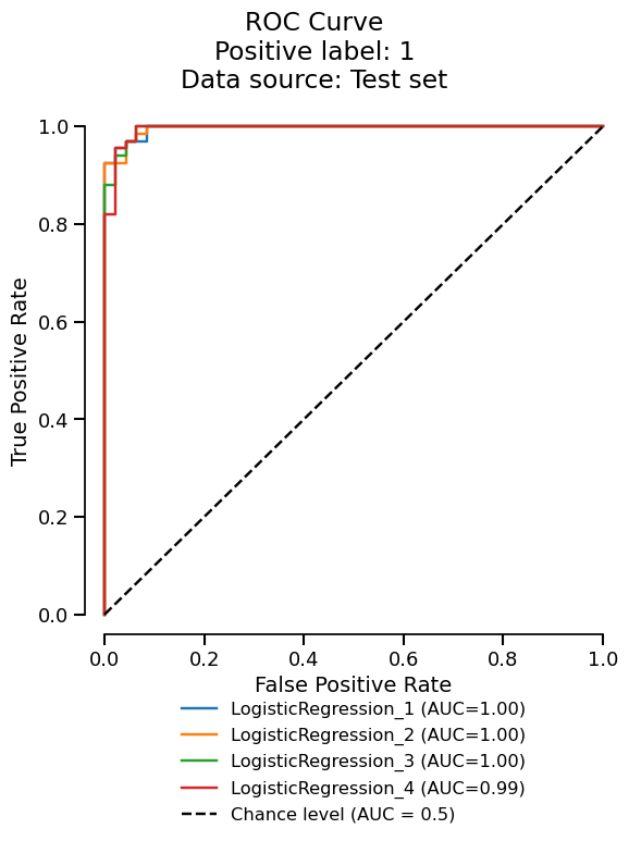
project.delete("example-project", workspace=tmp_path)
tmp_dir.cleanup()
Total running time of the script: (0 minutes 20.519 seconds)