Note
Go to the end to download the full example code.
Simplified experiment reporting#
This example shows how to leverage skore for reporting model evaluation and storing the results for further analysis.
We set some environment variables to avoid some spurious warnings related to parallelism.
import os

os.environ["POLARS_ALLOW_FORKING_THREAD"] = "1"
os.environ["TOKENIZERS_PARALLELISM"] = "true"
Creating a skore project and loading some data#
Let’s open a skore project in which we will be able to store artifacts from our experiments.
import skore

project = skore.open("my_project", create=True)
We use a skrub dataset that is non-trivial.
from skrub.datasets import fetch_employee_salaries

datasets = fetch_employee_salaries()
df, y = datasets.X, datasets.y
Let’s first have a condensed summary of the input data using a
skrub.TableReport.
from skrub import TableReport

table_report = TableReport(df)
table_report
From the table report, we can make a few observations:
The type of data is heterogeneous: we mainly have categorical and date-related features.
The year related to the
date_first_hiredcolumn is also present in thedatecolumn. Hence, we should beware of not creating twice the same feature during the feature engineering.By looking at the “Associations” tab of the table report, we observe that two features are holding the exact same information:
departmentanddepartment_name. Hence, during our feature engineering, we could potentially drop one of them if the final predictive model is sensitive to the collinearity.
We can store the report in the skore project so that we can easily retrieve it later without necessarily having to reload the dataset and recompute the report.
project.put("Input data summary", table_report)
In terms of target and thus the task that we want to solve, we are interested in predicting the salary of an employee given the previous features. We therefore have a regression task at end.
0        69222.18
1        97392.47
2       104717.28
3        52734.57
4        93396.00
          ...
9223     72094.53
9224    169543.85
9225    102736.52
9226    153747.50
9227     75484.08
Name: current_annual_salary, Length: 9228, dtype: float64
Modelling#
In a first attempt, we define a rather complex predictive model that uses a linear model as a base estimator.
import numpy as np
from sklearn.compose import make_column_transformer
from sklearn.pipeline import make_pipeline
from sklearn.preprocessing import OneHotEncoder, SplineTransformer
from sklearn.linear_model import RidgeCV
from skrub import DatetimeEncoder, ToDatetime, DropCols


def periodic_spline_transformer(period, n_splines=None, degree=3):
    if n_splines is None:
        n_splines = period
    n_knots = n_splines + 1  # periodic and include_bias is True
    return SplineTransformer(
        degree=degree,
        n_knots=n_knots,
        knots=np.linspace(0, period, n_knots).reshape(n_knots, 1),
        extrapolation="periodic",
        include_bias=True,
    )


categorical_features = [
    "gender",
    "department_name",
    "division",
    "assignment_category",
    "employee_position_title",
    "year_first_hired",
]
datetime_features = "date_first_hired"

date_encoder = make_pipeline(
    ToDatetime(),
    DatetimeEncoder(resolution="day", add_weekday=True, add_total_seconds=False),
    DropCols("date_first_hired_year"),
)

date_engineering = make_column_transformer(
    (periodic_spline_transformer(12, n_splines=6), ["date_first_hired_month"]),
    (periodic_spline_transformer(31, n_splines=15), ["date_first_hired_day"]),
    (periodic_spline_transformer(7, n_splines=3), ["date_first_hired_weekday"]),
)

feature_engineering_date = make_pipeline(date_encoder, date_engineering)

preprocessing = make_column_transformer(
    (feature_engineering_date, datetime_features),
    (OneHotEncoder(drop="if_binary", handle_unknown="ignore"), categorical_features),
)

model = make_pipeline(preprocessing, RidgeCV(alphas=np.logspace(-3, 3, 100)))
model
In the diagram above, we can see what how we performed our feature engineering:
For categorical features, we use a
OneHotEncoderto transform the categorical features. From the previous data exploration using aTableReport, from the “Stats” tab, one may have looked at the number of unique values and observed that we have feature with a large cardinality. In such cases, one-hot encoding might not be the best choice, but this is our starting point to get the ball rolling.Then, we have another transformation to encode the date features. We first split the date into multiple features (day, month, and year). Then, we apply a periodic spline transformation to each of the date features to capture the periodicity of the data.
Finally, we fit a
RidgeCVmodel.
Model evaluation using skore.CrossValidationReport#
First model#
Now, we want to evaluate this complex model via cross-validation (with 5 folds).
For that, we use skore’s CrossValidationReport to investigate the
performance of our model.
from skore import CrossValidationReport

report = CrossValidationReport(estimator=model, X=df, y=y, cv_splitter=5)
report.help()
  Processing cross-validation ━━━━━━━━━━━━━━━━━━━━━━━━━━━━━━━━━━━━━━━━ 100%
  for RidgeCV
╭──────────────────────── Tools to diagnose estimator RidgeCV ─────────────────────────╮
│ report                                                                               │
│ ├── .metrics                                                                         │
│ │   ├── .r2(...)               (↗︎)     - Compute the R² score.                       │
│ │   ├── .rmse(...)             (↘︎)     - Compute the root mean squared error.        │
│ │   ├── .custom_metric(...)            - Compute a custom metric.                    │
│ │   ├── .report_metrics(...)           - Report a set of metrics for our estimator.  │
│ │   └── .plot                                                                        │
│ │       └── .prediction_error(...)     - Plot the prediction error of a regression   │
│ │           model.                                                                   │
│ ├── .cache_predictions(...)            - Cache the predictions for sub-estimators    │
│ │   reports.                                                                         │
│ ├── .clear_cache(...)                  - Clear the cache.                            │
│ └── Attributes                                                                       │
│     ├── .X                                                                           │
│     ├── .y                                                                           │
│     ├── .estimator_                                                                  │
│     ├── .estimator_name_                                                             │
│     ├── .estimator_reports_                                                          │
│     └── .n_jobs                                                                      │
│                                                                                      │
│                                                                                      │
│ Legend:                                                                              │
│ (↗︎) higher is better (↘︎) lower is better                                             │
╰──────────────────────────────────────────────────────────────────────────────────────╯
We observe that the cross-validation report detected that we have a regression task and provides us with some metrics and plots that make sense for our specific problem at hand.
To accelerate any future computation (e.g. of a metric), we cache once and for all the predictions of our model. Note that we don’t necessarily need to cache the predictions as the report will compute them on the fly (if not cached) and cache them for us.
import warnings

with warnings.catch_warnings():
    # catch the warnings raised by the OneHotEncoder for seeing unknown categories
    # at transform time
    warnings.simplefilter(action="ignore", category=UserWarning)
    report.cache_predictions(n_jobs=3)
/home/thomas/Documents/workspace/probabl/skore/.venv/lib/python3.12/site-packages/sklearn/pipeline.py:62: FutureWarning:

This Pipeline instance is not fitted yet. Call 'fit' with appropriate arguments before using other methods such as transform, predict, etc. This will raise an error in 1.8 instead of the current warning.

  Cross-validation predictions ━━━━━━━━━━━━━━━━━━━━━━━━━━━━━━━━━━━━━━━━ 100%
  Caching predictions          ━━━━━━━━━━━━━━━━━━━━━━━━━━━━━━━━━━━━━━━━ 100%
  Caching predictions          ━━━━━━━━━━━━━━━━━━━━━━━━━━━━━━━━━━━━━━━━ 100%
  Caching predictions          ━━━━━━━━━━━━━━━━━━━━━━━━━━━━━━━━━━━━━━━━ 100%
  Caching predictions          ━━━━━━━━━━━━━━━━━━━━━━━━━━━━━━━━━━━━━━━━ 100%
  Caching predictions          ━━━━━━━━━━━━━━━━━━━━━━━━━━━━━━━━━━━━━━━━ 100%
To not lose this cross-validation report, let’s store it in our skore project.
project.put("Linear model report", report)
We can now have a look at the performance of the model with some standard metrics.
report.metrics.report_metrics(aggregate=["mean", "std"])
Compute metric for each split ━━━━━━━━━━━━━━━━━━━━━━━━━━━━━━━━━━━━━━━━ 100%
Second model#
Now that we have our first baseline model, we can try an out-of-the-box model:
skrub’s TableVectorizer that makes the feature engineering for us.
To deal with the high cardinality of the categorical features, we use a
TextEncoder that uses a language model and an embedding model to
encode the categorical features.
Finally, we use a HistGradientBoostingRegressor as a
base estimator that is a rather robust model.
from skrub import TableVectorizer, TextEncoder
from sklearn.ensemble import HistGradientBoostingRegressor
from sklearn.pipeline import make_pipeline

model = make_pipeline(
    TableVectorizer(high_cardinality=TextEncoder()),
    HistGradientBoostingRegressor(),
)
model
Let’s compute the cross-validation report for this model.
report = CrossValidationReport(estimator=model, X=df, y=y, cv_splitter=5, n_jobs=3)
report.help()
  Processing cross-validation       ━━━━━━━━━━━━━━━━━━━━━━━━━━━━━━━━━━━━━━━━ 100%
  for HistGradientBoostingRegressor
╭───────────── Tools to diagnose estimator HistGradientBoostingRegressor ──────────────╮
│ report                                                                               │
│ ├── .metrics                                                                         │
│ │   ├── .r2(...)               (↗︎)     - Compute the R² score.                       │
│ │   ├── .rmse(...)             (↘︎)     - Compute the root mean squared error.        │
│ │   ├── .custom_metric(...)            - Compute a custom metric.                    │
│ │   ├── .report_metrics(...)           - Report a set of metrics for our estimator.  │
│ │   └── .plot                                                                        │
│ │       └── .prediction_error(...)     - Plot the prediction error of a regression   │
│ │           model.                                                                   │
│ ├── .cache_predictions(...)            - Cache the predictions for sub-estimators    │
│ │   reports.                                                                         │
│ ├── .clear_cache(...)                  - Clear the cache.                            │
│ └── Attributes                                                                       │
│     ├── .X                                                                           │
│     ├── .y                                                                           │
│     ├── .estimator_                                                                  │
│     ├── .estimator_name_                                                             │
│     ├── .estimator_reports_                                                          │
│     └── .n_jobs                                                                      │
│                                                                                      │
│                                                                                      │
│ Legend:                                                                              │
│ (↗︎) higher is better (↘︎) lower is better                                             │
╰──────────────────────────────────────────────────────────────────────────────────────╯
We cache the predictions for later use.
report.cache_predictions(n_jobs=3)
Cross-validation predictions ━━━━━━━━━━━━━━━━━━━━━━━━━━━━━━━━━━━━━━━━ 100%
Caching predictions          ━━━━━━━━━━━━━━━━━━━━━━━━━━━━━━━━━━━━━━━━ 100%
Caching predictions          ━━━━━━━━━━━━━━━━━━━━━━━━━━━━━━━━━━━━━━━━ 100%
Caching predictions          ━━━━━━━━━━━━━━━━━━━━━━━━━━━━━━━━━━━━━━━━ 100%
Caching predictions          ━━━━━━━━━━━━━━━━━━━━━━━━━━━━━━━━━━━━━━━━ 100%
Caching predictions          ━━━━━━━━━━━━━━━━━━━━━━━━━━━━━━━━━━━━━━━━ 100%
We store the report in our skore project.
project.put("HGBDT model report", report)
We can now have a look at the performance of the model with some standard metrics.
report.metrics.report_metrics(aggregate=["mean", "std"])
Compute metric for each split ━━━━━━━━━━━━━━━━━━━━━━━━━━━━━━━━━━━━━━━━ 100%
Investigating the models#
At this stage, we might not been careful and have already overwritten the report and model from our first attempt. Hopefully, because we stored the reports in our skore project, we can easily retrieve them. So let’s retrieve the reports.
linear_model_report = project.get("Linear model report")
hgbdt_model_report = project.get("HGBDT model report")
Now that we retrieved the reports, we can make further comparison and build upon some usual pandas operations to concatenate the results.
import pandas as pd

results = pd.concat(
    [
        linear_model_report.metrics.report_metrics(aggregate=["mean", "std"]),
        hgbdt_model_report.metrics.report_metrics(aggregate=["mean", "std"]),
    ]
)
results
Compute metric for each split ━━━━━━━━━━━━━━━━━━━━━━━━━━━━━━━━━━━━━━━━ 100%
Compute metric for each split ━━━━━━━━━━━━━━━━━━━━━━━━━━━━━━━━━━━━━━━━ 100%
In addition, if we forgot to compute a specific metric
(e.g. mean_absolute_error()),
we can easily add it to the report, without re-training the model and even
without re-computing the predictions since they are cached internally in the report.
This allows us to save some potentially huge computation time.
from sklearn.metrics import mean_absolute_error

scoring = ["r2", "rmse", mean_absolute_error]
scoring_kwargs = {"response_method": "predict"}
scoring_names = ["R2", "RMSE", "MAE"]
results = pd.concat(
    [
        linear_model_report.metrics.report_metrics(
            scoring=scoring,
            scoring_kwargs=scoring_kwargs,
            scoring_names=scoring_names,
            aggregate=["mean", "std"],
        ),
        hgbdt_model_report.metrics.report_metrics(
            scoring=scoring,
            scoring_kwargs=scoring_kwargs,
            scoring_names=scoring_names,
            aggregate=["mean", "std"],
        ),
    ]
)
results
Compute metric for each split ━━━━━━━━━━━━━━━━━━━━━━━━━━━━━━━━━━━━━━━━ 100%
Compute metric for each split ━━━━━━━━━━━━━━━━━━━━━━━━━━━━━━━━━━━━━━━━ 100%
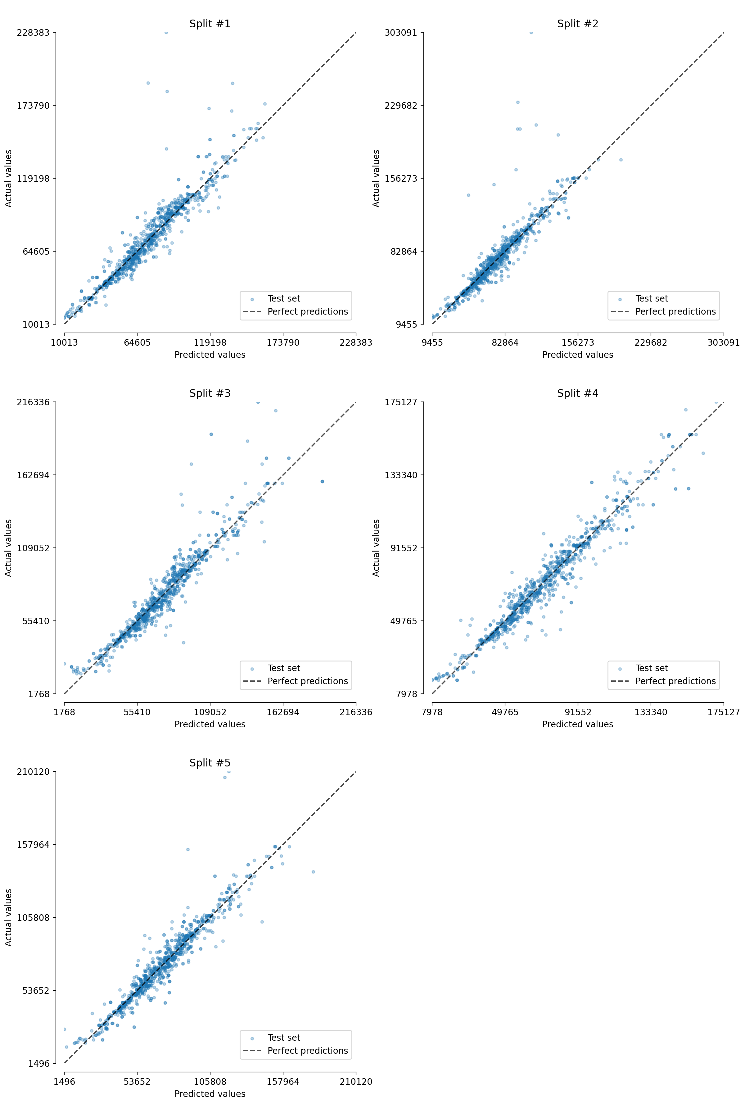
Finally, we can even get the individual EstimatorReport for each fold
from the cross-validation to make further analysis.
Here, we plot the actual vs predicted values for each fold.
from itertools import zip_longest
import matplotlib.pyplot as plt

fig, axs = plt.subplots(ncols=2, nrows=3, figsize=(12, 18))
for split_idx, (ax, estimator_report) in enumerate(
    zip_longest(axs.flatten(), linear_model_report.estimator_reports_)
):
    if estimator_report is None:
        ax.axis("off")
        continue
    estimator_report.metrics.plot.prediction_error(kind="actual_vs_predicted", ax=ax)
    ax.set_title(f"Split #{split_idx + 1}")
    ax.legend(loc="lower right")
plt.tight_layout()
Cleanup the project#
Let’s clear the skore project (to avoid any conflict with other documentation examples).
Total running time of the script: (4 minutes 7.740 seconds)