Cache mechanism

This example shows how EstimatorReport and CrossValidationReport use caching to speed up computations.

We set some environment variables to avoid some spurious warnings related to parallelism.

import os

os.environ["POLARS_ALLOW_FORKING_THREAD"] = "1"

Loading some data

First, we load a dataset from skrub. Our goal is to predict if a company paid a physician. The ultimate goal is to detect potential conflict of interest when it comes to the actual problem that we want to solve.

from skrub.datasets import fetch_open_payments

dataset = fetch_open_payments()
df = dataset.X
y = dataset.y

from skrub import TableReport

TableReport(df)

Please enable javascript

The skrub table reports need javascript to display correctly. If you are displaying a report in a Jupyter notebook and you see this message, you may need to re-execute the cell or to trust the notebook (button on the top right or "File > Trust notebook").

import pandas as pd

TableReport(pd.DataFrame(y))

Please enable javascript

The skrub table reports need javascript to display correctly. If you are displaying a report in a Jupyter notebook and you see this message, you may need to re-execute the cell or to trust the notebook (button on the top right or "File > Trust notebook").

The dataset has over 70,000 records with only categorical features. Some categories are not well defined.

Caching with EstimatorReport and CrossValidationReport

We use skrub to create a simple predictive model that handles our dataset’s challenges.

from skrub import tabular_learner

model = tabular_learner("classifier")
model

Pipeline(steps=[('tablevectorizer',
                 TableVectorizer(high_cardinality=MinHashEncoder(),
                                 low_cardinality=ToCategorical())),
                ('histgradientboostingclassifier',
                 HistGradientBoostingClassifier())])

In a Jupyter environment, please rerun this cell to show the HTML representation or trust the notebook.
On GitHub, the HTML representation is unable to render, please try loading this page with nbviewer.org.

This model handles all types of data: numbers, categories, dates, and missing values. Let’s train it on part of our dataset.

from skore import train_test_split

X_train, X_test, y_train, y_test = train_test_split(df, y, random_state=42)

╭───────────────────────────── HighClassImbalanceWarning ──────────────────────────────╮
│ It seems that you have a classification problem with a high class imbalance. In this │
│ case, using train_test_split may not be a good idea because of high variability in   │
│ the scores obtained on the test set. To tackle this challenge we suggest to use      │
│ skore's cross_validate function.                                                     │
╰──────────────────────────────────────────────────────────────────────────────────────╯
╭───────────────────────────────── ShuffleTrueWarning ─────────────────────────────────╮
│ We detected that the `shuffle` parameter is set to `True` either explicitly or from  │
│ its default value. In case of time-ordered events (even if they are independent),    │
│ this will result in inflated model performance evaluation because natural drift will │
│ not be taken into account. We recommend setting the shuffle parameter to `False` in  │
│ order to ensure the evaluation process is really representative of your production   │
│ release process.                                                                     │
╰──────────────────────────────────────────────────────────────────────────────────────╯

Caching the predictions for fast metric computation

First, we focus on EstimatorReport, as the same philosophy will apply to CrossValidationReport.

Let’s explore how EstimatorReport uses caching to speed up predictions. We start by training the model:

from skore import EstimatorReport

report = EstimatorReport(
    model, X_train=X_train, y_train=y_train, X_test=X_test, y_test=y_test
)
report.help()

╭──────────── Tools to diagnose estimator HistGradientBoostingClassifier ─────────────╮
│ report                                                                              │
│ ├── .metrics                                                                        │
│ │   ├── .accuracy(...)         (↗︎)     - Compute the accuracy score.                │
│ │   ├── .brier_score(...)      (↘︎)     - Compute the Brier score.                   │
│ │   ├── .log_loss(...)         (↘︎)     - Compute the log loss.                      │
│ │   ├── .precision(...)        (↗︎)     - Compute the precision score.               │
│ │   ├── .recall(...)           (↗︎)     - Compute the recall score.                  │
│ │   ├── .roc_auc(...)          (↗︎)     - Compute the ROC AUC score.                 │
│ │   ├── .custom_metric(...)            - Compute a custom metric.                   │
│ │   ├── .report_metrics(...)           - Report a set of metrics for our estimator. │
│ │   └── .plot                                                                       │
│ │       ├── .precision_recall(...)     - Plot the precision-recall curve.           │
│ │       └── .roc(...)                  - Plot the ROC curve.                        │
│ ├── .cache_predictions(...)            - Cache estimator's predictions.             │
│ ├── .clear_cache(...)                  - Clear the cache.                           │
│ └── Attributes                                                                      │
│     ├── .X_test                                                                     │
│     ├── .X_train                                                                    │
│     ├── .y_test                                                                     │
│     ├── .y_train                                                                    │
│     ├── .estimator_                                                                 │
│     └── .estimator_name_                                                            │
│                                                                                     │
│                                                                                     │
│ Legend:                                                                             │
│ (↗︎) higher is better (↘︎) lower is better                                            │
╰─────────────────────────────────────────────────────────────────────────────────────╯

We compute the accuracy on our test set and measure how long it takes:

import time

start = time.time()
result = report.metrics.accuracy()
end = time.time()
result

Metric	Accuracy (↗︎)
HistGradientBoostingClassifier	0.952257

print(f"Time taken: {end - start:.2f} seconds")

Time taken: 1.13 seconds

For comparison, here’s how scikit-learn computes the same accuracy score:

from sklearn.metrics import accuracy_score

start = time.time()
result = accuracy_score(report.y_test, report.estimator_.predict(report.X_test))
end = time.time()
result

0.9522566612289287

print(f"Time taken: {end - start:.2f} seconds")

Time taken: 1.12 seconds

Both approaches take similar time.

Now, watch what happens when we compute the accuracy again with our skore estimator report:

start = time.time()
result = report.metrics.accuracy()
end = time.time()
result

Metric	Accuracy (↗︎)
HistGradientBoostingClassifier	0.952257

print(f"Time taken: {end - start:.2f} seconds")

Time taken: 0.00 seconds

The second calculation is instant! This happens because the report saves previous calculations in its cache. Let’s look inside the cache:

report._cache

{(np.int64(7485932873459759447), 'predict', 'test'): array(['disallowed', 'disallowed', 'disallowed', ..., 'disallowed',
       'disallowed', 'disallowed'], shape=(18390,), dtype=object), (np.int64(7485932873459759447), 'accuracy_score', 'test'): 0.9522566612289287}

The cache stores predictions by type and data source. This means that computing metrics that use the same type of predictions will be faster. Let’s try the precision metric:

start = time.time()
result = report.metrics.precision()
end = time.time()
result

Metric	Precision (↗︎)
Class label	allowed	disallowed
HistGradientBoostingClassifier	0.682864	0.964221

print(f"Time taken: {end - start:.2f} seconds")

Time taken: 0.07 seconds

We observe that it takes only a few milliseconds to compute the precision because we don’t need to re-compute the predictions and only have to compute the precision metric itself. Since the predictions are the bottleneck in terms of computation time, we observe an interesting speedup.

Caching all the possible predictions at once

We can pre-compute all predictions at once using parallel processing:

report.cache_predictions(n_jobs=2)

Caching predictions ━━━━━━━━━━━━━━━━━━━━━━━━━━━━━━━━━━━━━━━━ 100%

Now, all possible predictions are stored. Any metric calculation will be much faster, even on different data (like the training set):

start = time.time()
result = report.metrics.log_loss(data_source="train")
end = time.time()
result

Metric	Log loss (↘︎)
HistGradientBoostingClassifier	0.098187

print(f"Time taken: {end - start:.2f} seconds")

Time taken: 0.14 seconds

Caching external data

The report can also work with external data. We use data_source="X_y" to indicate that we want to pass those external data.

start = time.time()
result = report.metrics.log_loss(data_source="X_y", X=X_test, y=y_test)
end = time.time()
result

Metric	Log loss (↘︎)
HistGradientBoostingClassifier	0.123282

print(f"Time taken: {end - start:.2f} seconds")

Time taken: 1.44 seconds

The first calculation of the above cell is slower than when using the internal train or test sets because it needs to compute a hash of the new data for later retrieval. Let’s calculate it again:

start = time.time()
result = report.metrics.log_loss(data_source="X_y", X=X_test, y=y_test)
end = time.time()
result

Metric	Log loss (↘︎)
HistGradientBoostingClassifier	0.123282

print(f"Time taken: {end - start:.2f} seconds")

Time taken: 0.16 seconds

It is much faster for the second time as the predictions are cached! The remaining time corresponds to the hash computation. Let’s compute the ROC AUC on the same data:

start = time.time()
result = report.metrics.roc_auc(data_source="X_y", X=X_test, y=y_test)
end = time.time()
result

Metric	ROC AUC (↗︎)
HistGradientBoostingClassifier	0.943145

print(f"Time taken: {end - start:.2f} seconds")

Time taken: 0.20 seconds

We observe that the computation is already efficient because it boils down to two computations: the hash of the data and the ROC-AUC metric. We save a lot of time because we don’t need to re-compute the predictions.

Caching for plotting

The cache also speeds up plots. Let’s create a ROC curve:

import matplotlib.pyplot as plt

start = time.time()
display = report.metrics.plot.roc(pos_label="allowed")
end = time.time()
plt.tight_layout()

print(f"Time taken: {end - start:.2f} seconds")

Time taken: 0.02 seconds

The second plot is instant because it uses cached data:

start = time.time()
display = report.metrics.plot.roc(pos_label="allowed")
end = time.time()
plt.tight_layout()

print(f"Time taken: {end - start:.2f} seconds")

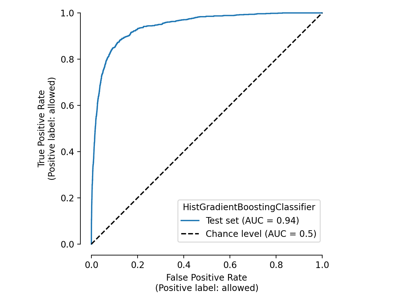
Time taken: 0.02 seconds

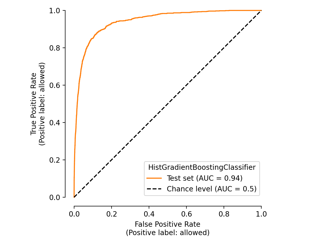
We only use the cache to retrieve the display object and not directly the matplotlib figure. It means that we can still customize the cached plot before displaying it:

display.plot(roc_curve_kwargs={"color": "tab:orange"})
plt.tight_layout()

Be aware that we can clear the cache if we want to:

report.clear_cache()
report._cache

{}

It means that nothing is stored anymore in the cache.

Caching with CrossValidationReport

CrossValidationReport uses the same caching system for each fold in cross-validation by leveraging the previous EstimatorReport:

from skore import CrossValidationReport

report = CrossValidationReport(model, X=df, y=y, cv_splitter=5, n_jobs=2)
report.help()

  Processing cross-validation        ━━━━━━━━━━━━━━━━━━━━━━━━━━━━━━━━━━━━━━━━ 100%
  for HistGradientBoostingClassifier
╭───────────── Tools to diagnose estimator HistGradientBoostingClassifier ─────────────╮
│ report                                                                               │
│ ├── .metrics                                                                         │
│ │   ├── .accuracy(...)         (↗︎)     - Compute the accuracy score.                 │
│ │   ├── .brier_score(...)      (↘︎)     - Compute the Brier score.                    │
│ │   ├── .log_loss(...)         (↘︎)     - Compute the log loss.                       │
│ │   ├── .precision(...)        (↗︎)     - Compute the precision score.                │
│ │   ├── .recall(...)           (↗︎)     - Compute the recall score.                   │
│ │   ├── .roc_auc(...)          (↗︎)     - Compute the ROC AUC score.                  │
│ │   ├── .custom_metric(...)            - Compute a custom metric.                    │
│ │   ├── .report_metrics(...)           - Report a set of metrics for our estimator.  │
│ │   └── .plot                                                                        │
│ │       ├── .precision_recall(...)     - Plot the precision-recall curve.            │
│ │       └── .roc(...)                  - Plot the ROC curve.                         │
│ ├── .cache_predictions(...)            - Cache the predictions for sub-estimators    │
│ │   reports.                                                                         │
│ ├── .clear_cache(...)                  - Clear the cache.                            │
│ └── Attributes                                                                       │
│     ├── .X                                                                           │
│     ├── .y                                                                           │
│     ├── .estimator_                                                                  │
│     ├── .estimator_name_                                                             │
│     ├── .estimator_reports_                                                          │
│     └── .n_jobs                                                                      │
│                                                                                      │
│                                                                                      │
│ Legend:                                                                              │
│ (↗︎) higher is better (↘︎) lower is better                                             │
╰──────────────────────────────────────────────────────────────────────────────────────╯

We can pre-compute all predictions at once using parallel processing:

report.cache_predictions(n_jobs=2)

Cross-validation predictions ━━━━━━━━━━━━━━━━━━━━━━━━━━━━━━━━━━━━━━━━ 100%
Caching predictions          ━━━━━━━━━━━━━━━━━━━━━━━━━━━━━━━━━━━━━━━━ 100%
Caching predictions          ━━━━━━━━━━━━━━━━━━━━━━━━━━━━━━━━━━━━━━━━ 100%
Caching predictions          ━━━━━━━━━━━━━━━━━━━━━━━━━━━━━━━━━━━━━━━━ 100%
Caching predictions          ━━━━━━━━━━━━━━━━━━━━━━━━━━━━━━━━━━━━━━━━ 100%
Caching predictions          ━━━━━━━━━━━━━━━━━━━━━━━━━━━━━━━━━━━━━━━━ 100%

Now, all possible predictions are stored. Any metric calculation will be much faster, even on different data, as we showed for the EstimatorReport.

start = time.time()
result = report.metrics.report_metrics(aggregate=["mean", "std"])
end = time.time()
result

Compute metric for each split ━━━━━━━━━━━━━━━━━━━━━━━━━━━━━━━━━━━━━━━━ 100%

	Metric	Precision (↗︎)		Recall (↗︎)		ROC AUC (↗︎)	Brier score (↘︎)
	Class label	allowed	disallowed	allowed	disallowed
HistGradientBoostingClassifier	mean	0.402622	0.959575	0.422807	0.942157	0.862601	0.069934
	std	0.136700	0.004676	0.091438	0.054469	0.039124	0.041601

print(f"Time taken: {end - start:.2f} seconds")

Time taken: 0.59 seconds

Hence, we observe the same type of behaviour as we previously exposed.