Note
Go to the end to download the full example code.
Skore: getting started#
This getting started guide illustrates how to use skore and why:
Track your ML/DS results using skore’s
Project(for storage).Machine learning diagnostics: get assistance when developing your ML/DS projects to avoid common pitfalls and follow recommended practices.
skore.EstimatorReport: get an insightful report for your estimatorskore.CrossValidationReport: get an insightful report for your cross-validation resultsskore.train_test_split(): get diagnostics when splitting your data
Tracking: skore project#
A key feature of skore is its Project that allows to store
items of many types.
Setup: creating and loading a skore project#
Let’s start by creating a skore project directory named my_project.skore in our
current directory.
import skore

my_project = skore.open("my_project", create=True)
Now that the project exists, we can write some Python code (in the same
directory) to add (put()) some useful items in it,
with a key-value convention:
my_project.put("my_int", 3)
We can retrieve the value of an item:
my_project.get("my_int")
3
Skore project: storing some items#
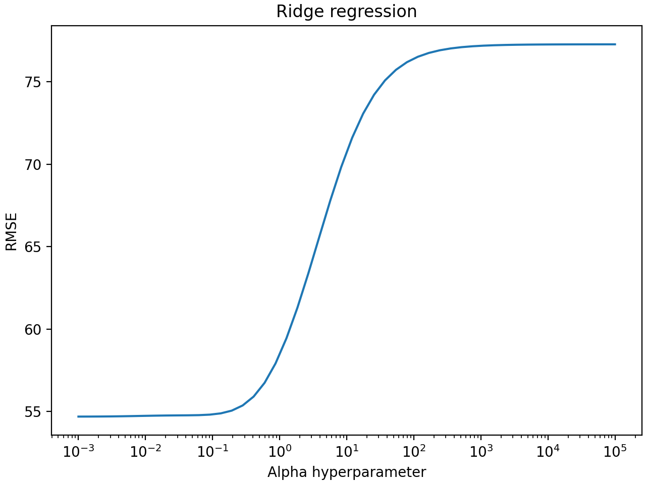
As an illustration of the usage of the skore project with a machine learning motivation, let us perform a hyperparameter sweep and store relevant information in the skore project.
We search for the alpha hyperparameter of a Ridge regression on the
Diabetes dataset:
import numpy as np
from sklearn.datasets import load_diabetes
from sklearn.linear_model import Ridge
from sklearn.model_selection import GridSearchCV

X, y = load_diabetes(return_X_y=True)

gs_cv = GridSearchCV(
    Ridge(),
    param_grid={"alpha": np.logspace(-3, 5, 50)},
    scoring="neg_root_mean_squared_error",
)
gs_cv.fit(X, y)
Now, we store the hyperparameter’s metrics in a dataframe and make a custom plot:
import pandas as pd

df = pd.DataFrame(gs_cv.cv_results_)
df.insert(len(df.columns), "rmse", -df["mean_test_score"].values)
df[["param_alpha", "rmse"]].head()
import matplotlib.pyplot as plt

fig = plt.figure(layout="constrained")
plt.plot(df["param_alpha"], df["rmse"])
plt.xscale("log")
plt.xlabel("Alpha hyperparameter")
plt.ylabel("RMSE")
plt.title("Ridge regression")
plt.show()
Finally, we store these relevant items in our skore project, so that we can visualize them later:
my_project.put("my_gs_cv", gs_cv)
my_project.put("my_df", df)
my_project.put("my_fig", fig)
See also
For more information about the functionalities and the different types
of items that we can store in a skore Project,
see Working with projects.
Tracking the history of items#
Suppose we store several values for a same item called my_key_metric:
my_project.put("my_key_metric", 4)

my_project.put("my_key_metric", 9)

my_project.put("my_key_metric", 16)
Skore does not overwrite items with the same name (key): instead, it stores their history so that nothing is lost.
These tracking functionalities are very useful to:
never lose some key machine learning metrics,
and observe the evolution over time / runs.
See also
For more information about the tracking of items using their history, see Tracking items.
Machine learning diagnostics and evaluation#
Skore re-implements or wraps some key scikit-learn class / functions to automatically provide diagnostics and checks when using them, as a way to facilitate good practices and avoid common pitfalls.
Model evaluation with skore#
In order to assist its users when programming, skore has implemented a
skore.EstimatorReport class.
Let us load some synthetic data and get the estimator report for a
LogisticRegression:
from sklearn.datasets import make_classification
from sklearn.linear_model import LogisticRegression
from sklearn.model_selection import train_test_split

from skore import EstimatorReport

X, y = make_classification(n_classes=2, n_samples=100_000, n_informative=4)
X_train, X_test, y_train, y_test = train_test_split(X, y, random_state=0)

clf = LogisticRegression()

est_report = EstimatorReport(
    clf, X_train=X_train, X_test=X_test, y_train=y_train, y_test=y_test
)
Now, we can display the help tree to see all the insights that are available to us given that we are doing binary classification:
╭────────────────── Tools to diagnose estimator LogisticRegression ───────────────────╮
│ report                                                                              │
│ ├── .metrics                                                                        │
│ │   ├── .accuracy(...)         (↗︎)     - Compute the accuracy score.                │
│ │   ├── .brier_score(...)      (↘︎)     - Compute the Brier score.                   │
│ │   ├── .log_loss(...)         (↘︎)     - Compute the log loss.                      │
│ │   ├── .precision(...)        (↗︎)     - Compute the precision score.               │
│ │   ├── .recall(...)           (↗︎)     - Compute the recall score.                  │
│ │   ├── .roc_auc(...)          (↗︎)     - Compute the ROC AUC score.                 │
│ │   ├── .custom_metric(...)            - Compute a custom metric.                   │
│ │   ├── .report_metrics(...)           - Report a set of metrics for our estimator. │
│ │   └── .plot                                                                       │
│ │       ├── .precision_recall(...)     - Plot the precision-recall curve.           │
│ │       └── .roc(...)                  - Plot the ROC curve.                        │
│ ├── .cache_predictions(...)            - Cache estimator's predictions.             │
│ ├── .clear_cache(...)                  - Clear the cache.                           │
│ └── Attributes                                                                      │
│     ├── .X_test                                                                     │
│     ├── .X_train                                                                    │
│     ├── .y_test                                                                     │
│     ├── .y_train                                                                    │
│     ├── .estimator_                                                                 │
│     └── .estimator_name_                                                            │
│                                                                                     │
│                                                                                     │
│ Legend:                                                                             │
│ (↗︎) higher is better (↘︎) lower is better                                            │
╰─────────────────────────────────────────────────────────────────────────────────────╯
We can get the report metrics that was computed for us:
df_est_report_metrics = est_report.metrics.report_metrics()
df_est_report_metrics
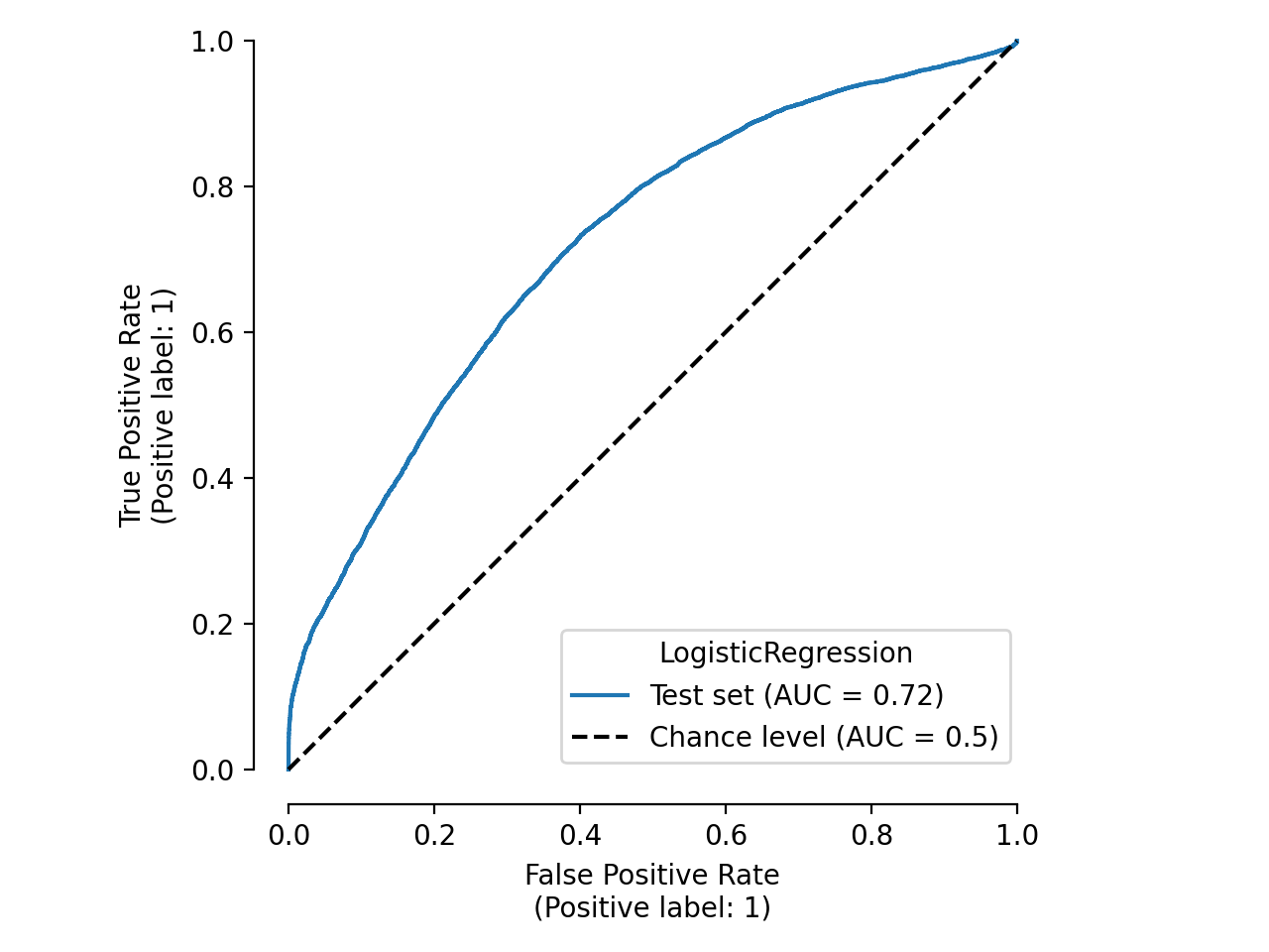
We can also plot the ROC curve that was generated for us:
import matplotlib.pyplot as plt

roc_plot = est_report.metrics.plot.roc()
roc_plot
plt.tight_layout()
See also
For more information about the motivation and usage of
skore.EstimatorReport, see Get insights from any scikit-learn estimator.
Cross-validation with skore#
skore has also implemented a skore.CrossValidationReport class that contains
several skore.EstimatorReport for each fold.
from skore import CrossValidationReport

cv_report = CrossValidationReport(clf, X, y, cv_splitter=5)
Processing cross-validation ━━━━━━━━━━━━━━━━━━━━━━━━━━━━━━━━━━━━━━━━ 100%
for LogisticRegression
We display the cross-validation report helper:
╭─────────────────── Tools to diagnose estimator LogisticRegression ───────────────────╮
│ report                                                                               │
│ ├── .metrics                                                                         │
│ │   ├── .accuracy(...)         (↗︎)     - Compute the accuracy score.                 │
│ │   ├── .brier_score(...)      (↘︎)     - Compute the Brier score.                    │
│ │   ├── .log_loss(...)         (↘︎)     - Compute the log loss.                       │
│ │   ├── .precision(...)        (↗︎)     - Compute the precision score.                │
│ │   ├── .recall(...)           (↗︎)     - Compute the recall score.                   │
│ │   ├── .roc_auc(...)          (↗︎)     - Compute the ROC AUC score.                  │
│ │   ├── .custom_metric(...)            - Compute a custom metric.                    │
│ │   ├── .report_metrics(...)           - Report a set of metrics for our estimator.  │
│ │   └── .plot                                                                        │
│ │       ├── .precision_recall(...)     - Plot the precision-recall curve.            │
│ │       └── .roc(...)                  - Plot the ROC curve.                         │
│ ├── .cache_predictions(...)            - Cache the predictions for sub-estimators    │
│ │   reports.                                                                         │
│ ├── .clear_cache(...)                  - Clear the cache.                            │
│ └── Attributes                                                                       │
│     ├── .X                                                                           │
│     ├── .y                                                                           │
│     ├── .estimator_                                                                  │
│     ├── .estimator_name_                                                             │
│     ├── .estimator_reports_                                                          │
│     └── .n_jobs                                                                      │
│                                                                                      │
│                                                                                      │
│ Legend:                                                                              │
│ (↗︎) higher is better (↘︎) lower is better                                             │
╰──────────────────────────────────────────────────────────────────────────────────────╯
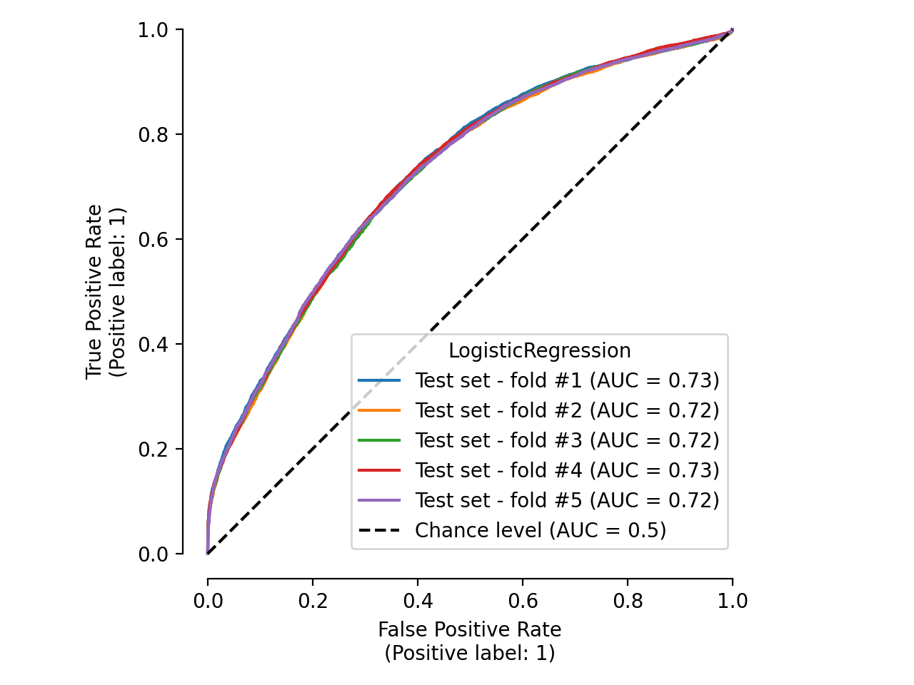
We display the metrics for each fold:
df_cv_report_metrics = cv_report.metrics.report_metrics()
df_cv_report_metrics
Compute metric for each split ━━━━━━━━━━━━━━━━━━━━━━━━━━━━━━━━━━━━━━━━ 100%
We display the ROC curves for each fold:
roc_plot = cv_report.metrics.plot.roc()
roc_plot
plt.tight_layout()
Computing predictions for display ━━━━━━━━━━━━━━━━━━━━━━━━━━━━━━━━━━━━━━━━ 100%
See also
For more information about the motivation and usage of
skore.CrossValidationReport, see Simplified experiment reporting.
Train-test split with skore#
Skore has implemented a skore.train_test_split() function that wraps
scikit-learn’s sklearn.model_selection.train_test_split().
Let us load a dataset containing some time series data:
from skrub.datasets import fetch_employee_salaries

dataset = fetch_employee_salaries()
X, y = dataset.X, dataset.y
X["date_first_hired"] = pd.to_datetime(X["date_first_hired"])
X.head(2)
We can observe that there is a date_first_hired which is time-based.
Now, let us apply skore.train_test_split() on this data:
╭─────────────────────────────── TimeBasedColumnWarning ───────────────────────────────╮
│ We detected some time-based columns (column "date_first_hired") in your data. We     │
│ recommend using scikit-learn's TimeSeriesSplit instead of train_test_split.          │
│ Otherwise you might train on future data to predict the past, or get inflated model  │
│ performance evaluation because natural drift will not be taken into account.         │
╰──────────────────────────────────────────────────────────────────────────────────────╯
We get a TimeBasedColumnWarning advising us to use
sklearn.model_selection.TimeSeriesSplit instead!
Indeed, we should not shuffle time-ordered data!
See also
More methodological advice is available.
For more information about the motivation and usage of
skore.train_test_split(), see Train-test split.
Stay tuned!
These are only the initial features: skore is a work in progress and aims to be an end-to-end library for data scientists.
Feedbacks are welcome: please feel free to join our Discord or create an issue.
Cleanup the project#
Let’s clear the skore project (to avoid any conflict with other documentation examples).
Total running time of the script: (0 minutes 4.846 seconds)