Note
Go to the end to download the full example code.
Simplified experiment reporting#
This example shows how to leverage skore for reporting model evaluation and storing the results for further analysis.
We set some environment variables to avoid some spurious warnings related to parallelism.
import os

os.environ["POLARS_ALLOW_FORKING_THREAD"] = "1"
os.environ["TOKENIZERS_PARALLELISM"] = "true"
Creating a skore project and loading some data#
We use a skrub dataset that is non-trivial.
from skrub.datasets import fetch_employee_salaries

datasets = fetch_employee_salaries()
df, y = datasets.X, datasets.y
Let’s first have a condensed summary of the input data using a
skrub.TableReport.
from skrub import TableReport

table_report = TableReport(df)
table_report
From the table report, we can make a few observations:
The type of data is heterogeneous: we mainly have categorical and date-related features.
The year related to the
date_first_hiredcolumn is also present in thedatecolumn. Hence, we should beware of not creating twice the same feature during the feature engineering.By looking at the “Associations” tab of the table report, we observe that two features are holding the exact same information:
departmentanddepartment_name. Hence, during our feature engineering, we could potentially drop one of them if the final predictive model is sensitive to the collinearity.When looking at the “Stats” tab, we observe that the
divisionandemployee_position_titleare two features containing a large number of categories. It is something that we should consider in our feature engineering.
In terms of target and thus the task that we want to solve, we are interested in predicting the salary of an employee given the previous features. We therefore have a regression task at end.
0        69222.18
1        97392.47
2       104717.28
3        52734.57
4        93396.00
          ...
9223     72094.53
9224    169543.85
9225    102736.52
9226    153747.50
9227     75484.08
Name: current_annual_salary, Length: 9228, dtype: float64
Tree-based model#
Let’s start by creating a tree-based model using some out-of-the-box tools.
For feature engineering we use skrub’s TableVectorizer.
To deal with the high cardinality of the categorical features, we use a
TextEncoder that uses a language model and an embedding model to
encode the categorical features.
Finally, we use a HistGradientBoostingRegressor as a
base estimator that is a rather robust model.
Modelling#
from skrub import TableVectorizer, TextEncoder
from sklearn.ensemble import HistGradientBoostingRegressor
from sklearn.pipeline import make_pipeline

model = make_pipeline(
    TableVectorizer(high_cardinality=TextEncoder()),
    HistGradientBoostingRegressor(),
)
model
Evaluation#
Let us compute the cross-validation report for this model using
skore.CrossValidationReport:
from skore import CrossValidationReport

hgbt_model_report = CrossValidationReport(
    estimator=model, X=df, y=y, cv_splitter=5, n_jobs=4
)
hgbt_model_report.help()
╭───────────── Tools to diagnose estimator HistGradientBoostingRegressor ──────────────╮
│ CrossValidationReport                                                                │
│ ├── .metrics                                                                         │
│ │   ├── .prediction_error(...)         - Plot the prediction error of a regression   │
│ │   │   model.                                                                       │
│ │   ├── .r2(...)               (↗︎)     - Compute the R² score.                       │
│ │   ├── .rmse(...)             (↘︎)     - Compute the root mean squared error.        │
│ │   ├── .timings(...)                  - Get all measured processing times related   │
│ │   │   to the estimator.                                                            │
│ │   ├── .custom_metric(...)            - Compute a custom metric.                    │
│ │   └── .summarize(...)                - Report a set of metrics for our estimator.  │
│ ├── .cache_predictions(...)            - Cache the predictions for sub-estimators    │
│ │   reports.                                                                         │
│ ├── .clear_cache(...)                  - Clear the cache.                            │
│ ├── .get_predictions(...)              - Get estimator's predictions.                │
│ └── Attributes                                                                       │
│     ├── .X                             - The data to fit                             │
│     ├── .y                             - The target variable to try to predict in    │
│     │   the case of supervised learning                                              │
│     ├── .cv_splitter                   - Determines the cross-validation splitting   │
│     │   strategy                                                                     │
│     ├── .estimator                     - Estimator to make the cross-validation      │
│     │   report from                                                                  │
│     ├── .estimator_                    - The cloned or copied estimator              │
│     ├── .estimator_name_               - The name of the estimator                   │
│     ├── .estimator_reports_            - The estimator reports for each split        │
│     ├── .n_jobs                        - Number of jobs to run in parallel           │
│     └── .pos_label                     - For binary classification, the positive     │
│         class                                                                        │
│                                                                                      │
│                                                                                      │
│ Legend:                                                                              │
│ (↗︎) higher is better (↘︎) lower is better                                             │
╰──────────────────────────────────────────────────────────────────────────────────────╯
We cache the predictions for later use.
hgbt_model_report.cache_predictions(n_jobs=4)
We can now have a look at the performance of the model with some standard metrics.
hgbt_model_report.metrics.summarize()
skore.MetricsSummaryDisplay(...)
Linear model#
Now that we have established a first model that serves as a baseline, we shall proceed to define a quite complex linear model (a pipeline with a complex feature engineering that uses a linear model as the base estimator).
Modelling#
import numpy as np
from sklearn.compose import make_column_transformer
from sklearn.pipeline import make_pipeline
from sklearn.preprocessing import OneHotEncoder, SplineTransformer
from sklearn.linear_model import RidgeCV
from skrub import DatetimeEncoder, ToDatetime, DropCols, GapEncoder


def periodic_spline_transformer(period, n_splines=None, degree=3):
    if n_splines is None:
        n_splines = period
    n_knots = n_splines + 1  # periodic and include_bias is True
    return SplineTransformer(
        degree=degree,
        n_knots=n_knots,
        knots=np.linspace(0, period, n_knots).reshape(n_knots, 1),
        extrapolation="periodic",
        include_bias=True,
    )


one_hot_features = ["gender", "department_name", "assignment_category"]
datetime_features = "date_first_hired"

date_encoder = make_pipeline(
    ToDatetime(),
    DatetimeEncoder(resolution="day", add_weekday=True, add_total_seconds=False),
    DropCols("date_first_hired_year"),
)

date_engineering = make_column_transformer(
    (periodic_spline_transformer(12, n_splines=6), ["date_first_hired_month"]),
    (periodic_spline_transformer(31, n_splines=15), ["date_first_hired_day"]),
    (periodic_spline_transformer(7, n_splines=3), ["date_first_hired_weekday"]),
)

feature_engineering_date = make_pipeline(date_encoder, date_engineering)

preprocessing = make_column_transformer(
    (feature_engineering_date, datetime_features),
    (OneHotEncoder(drop="if_binary", handle_unknown="ignore"), one_hot_features),
    (GapEncoder(n_components=100), "division"),
    (GapEncoder(n_components=100), "employee_position_title"),
)

model = make_pipeline(preprocessing, RidgeCV(alphas=np.logspace(-3, 3, 100)))
model
Pipeline(steps=[('columntransformer',
                 ColumnTransformer(transformers=[('pipeline',
                                                  Pipeline(steps=[('pipeline',
                                                                   Pipeline(steps=[('todatetime',
                                                                                    ToDatetime()),
                                                                                   ('datetimeencoder',
                                                                                    DatetimeEncoder(add_total_seconds=False,
                                                                                                    add_weekday=True,
                                                                                                    resolution='day')),
                                                                                   ('dropcols',
                                                                                    DropCols(cols='date_first_hired_year'))])),
                                                                  ('columntransformer',
                                                                   ColumnTransformer(transfor...
       4.03701726e+01, 4.64158883e+01, 5.33669923e+01, 6.13590727e+01,
       7.05480231e+01, 8.11130831e+01, 9.32603347e+01, 1.07226722e+02,
       1.23284674e+02, 1.41747416e+02, 1.62975083e+02, 1.87381742e+02,
       2.15443469e+02, 2.47707636e+02, 2.84803587e+02, 3.27454916e+02,
       3.76493581e+02, 4.32876128e+02, 4.97702356e+02, 5.72236766e+02,
       6.57933225e+02, 7.56463328e+02, 8.69749003e+02, 1.00000000e+03])))])
In the diagram above, we can see what how we performed our feature engineering:
For categorical features, we use two approaches: if the number of categories is relatively small, we use a
OneHotEncoderand if the number of categories is large, we use aGapEncoderthat was designed to deal with high cardinality categorical features.Then, we have another transformation to encode the date features. We first split the date into multiple features (day, month, and year). Then, we apply a periodic spline transformation to each of the date features to capture the periodicity of the data.
Finally, we fit a
RidgeCVmodel.
Evaluation#
Now, we want to evaluate this linear model via cross-validation (with 5 folds).
For that, we use skore’s CrossValidationReport to investigate the
performance of our model.
linear_model_report = CrossValidationReport(
    estimator=model, X=df, y=y, cv_splitter=5, n_jobs=4
)
linear_model_report.help()
╭──────────────────────── Tools to diagnose estimator RidgeCV ─────────────────────────╮
│ CrossValidationReport                                                                │
│ ├── .metrics                                                                         │
│ │   ├── .prediction_error(...)         - Plot the prediction error of a regression   │
│ │   │   model.                                                                       │
│ │   ├── .r2(...)               (↗︎)     - Compute the R² score.                       │
│ │   ├── .rmse(...)             (↘︎)     - Compute the root mean squared error.        │
│ │   ├── .timings(...)                  - Get all measured processing times related   │
│ │   │   to the estimator.                                                            │
│ │   ├── .custom_metric(...)            - Compute a custom metric.                    │
│ │   └── .summarize(...)                - Report a set of metrics for our estimator.  │
│ ├── .cache_predictions(...)            - Cache the predictions for sub-estimators    │
│ │   reports.                                                                         │
│ ├── .clear_cache(...)                  - Clear the cache.                            │
│ ├── .get_predictions(...)              - Get estimator's predictions.                │
│ └── Attributes                                                                       │
│     ├── .X                             - The data to fit                             │
│     ├── .y                             - The target variable to try to predict in    │
│     │   the case of supervised learning                                              │
│     ├── .cv_splitter                   - Determines the cross-validation splitting   │
│     │   strategy                                                                     │
│     ├── .estimator                     - Estimator to make the cross-validation      │
│     │   report from                                                                  │
│     ├── .estimator_                    - The cloned or copied estimator              │
│     ├── .estimator_name_               - The name of the estimator                   │
│     ├── .estimator_reports_            - The estimator reports for each split        │
│     ├── .n_jobs                        - Number of jobs to run in parallel           │
│     └── .pos_label                     - For binary classification, the positive     │
│         class                                                                        │
│                                                                                      │
│                                                                                      │
│ Legend:                                                                              │
│ (↗︎) higher is better (↘︎) lower is better                                             │
╰──────────────────────────────────────────────────────────────────────────────────────╯
We observe that the cross-validation report detected that we have a regression task and provides us with some metrics and plots that make sense for our specific problem at hand.
To accelerate any future computation (e.g. of a metric), we cache once and for all the predictions of our model. Note that we do not necessarily need to cache the predictions as the report will compute them on the fly (if not cached) and cache them for us.
import warnings

with warnings.catch_warnings():
    warnings.simplefilter(action="ignore", category=FutureWarning)
    linear_model_report.cache_predictions(n_jobs=4)
We can now have a look at the performance of the model with some standard metrics.
linear_model_report.metrics.summarize(indicator_favorability=True)
skore.MetricsSummaryDisplay(...)
Comparing the models#
Now that we cross-validated our models, we can make some further comparison using the
skore.ComparisonReport:
from skore import ComparisonReport

comparator = ComparisonReport([hgbt_model_report, linear_model_report])
comparator.metrics.summarize(indicator_favorability=True)
skore.MetricsSummaryDisplay(...)
In addition, if we forgot to compute a specific metric
(e.g. mean_absolute_error()),
we can easily add it to the report, without re-training the model and even
without re-computing the predictions since they are cached internally in the report.
This allows us to save some potentially huge computation time.
from sklearn.metrics import mean_absolute_error

scoring = ["r2", "rmse", mean_absolute_error]
scoring_kwargs = {"response_method": "predict"}
scoring_names = ["R²", "RMSE", "MAE"]

comparator.metrics.summarize(
    scoring=scoring,
    scoring_kwargs=scoring_kwargs,
    scoring_names=scoring_names,
)
skore.MetricsSummaryDisplay(...)
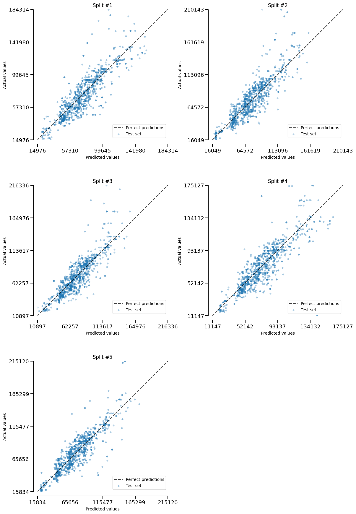
Finally, we can even get a deeper understanding by analyzing each fold in the
CrossValidationReport.
Here, we plot the actual-vs-predicted values for each fold.
import matplotlib.pyplot as plt

linear_model_report.metrics.prediction_error().plot(kind="actual_vs_predicted")

plt.tight_layout()
Total running time of the script: (1 minutes 31.784 seconds)