Cache mechanism

This example shows how EstimatorReport and CrossValidationReport use caching to speed up computations.

Loading some data

First, we load a dataset from skrub. Our goal is to predict if a company paid a physician. The ultimate goal is to detect potential conflict of interest when it comes to the actual problem that we want to solve.

from skrub.datasets import fetch_open_payments

dataset = fetch_open_payments()
df = dataset.X
y = dataset.y

from skrub import TableReport

TableReport(df)

Please enable javascript

The skrub table reports need javascript to display correctly. If you are displaying a report in a Jupyter notebook and you see this message, you may need to re-execute the cell or to trust the notebook (button on the top right or "File > Trust notebook").

import pandas as pd

TableReport(pd.DataFrame(y))

Please enable javascript

The skrub table reports need javascript to display correctly. If you are displaying a report in a Jupyter notebook and you see this message, you may need to re-execute the cell or to trust the notebook (button on the top right or "File > Trust notebook").

The dataset has over 70,000 records with only categorical features. Some categories are not well defined.

Caching with EstimatorReport and CrossValidationReport

We use skrub to create a simple predictive model that handles our dataset’s challenges.

from skrub import tabular_learner

model = tabular_learner("classifier")
model

/opt/hostedtoolcache/Python/3.12.11/x64/lib/python3.12/site-packages/skrub/_tabular_pipeline.py:75: FutureWarning:

tabular_learner will be deprecated in the next release. Equivalent functionality is available in skrub.tabular_pipeline.

Pipeline(steps=[('tablevectorizer',
                 TableVectorizer(low_cardinality=ToCategorical())),
                ('histgradientboostingclassifier',
                 HistGradientBoostingClassifier())])

In a Jupyter environment, please rerun this cell to show the HTML representation or trust the notebook.
On GitHub, the HTML representation is unable to render, please try loading this page with nbviewer.org.

This model handles all types of data: numbers, categories, dates, and missing values. Let’s train it on part of our dataset.

from skore import train_test_split

X_train, X_test, y_train, y_test = train_test_split(df, y, random_state=42)
# Let's keep a completely separate dataset
X_train, X_external, y_train, y_external = train_test_split(
    X_train, y_train, random_state=42
)

╭───────────────────────────── HighClassImbalanceWarning ──────────────────────────────╮
│ It seems that you have a classification problem with a high class imbalance. In this │
│ case, using train_test_split may not be a good idea because of high variability in   │
│ the scores obtained on the test set. To tackle this challenge we suggest to use      │
│ skore's CrossValidationReport with the `splitter` parameter of your choice.          │
╰──────────────────────────────────────────────────────────────────────────────────────╯
╭───────────────────────────────── ShuffleTrueWarning ─────────────────────────────────╮
│ We detected that the `shuffle` parameter is set to `True` either explicitly or from  │
│ its default value. In case of time-ordered events (even if they are independent),    │
│ this will result in inflated model performance evaluation because natural drift will │
│ not be taken into account. We recommend setting the shuffle parameter to `False` in  │
│ order to ensure the evaluation process is really representative of your production   │
│ release process.                                                                     │
╰──────────────────────────────────────────────────────────────────────────────────────╯
╭───────────────────────────── HighClassImbalanceWarning ──────────────────────────────╮
│ It seems that you have a classification problem with a high class imbalance. In this │
│ case, using train_test_split may not be a good idea because of high variability in   │
│ the scores obtained on the test set. To tackle this challenge we suggest to use      │
│ skore's CrossValidationReport with the `splitter` parameter of your choice.          │
╰──────────────────────────────────────────────────────────────────────────────────────╯
╭───────────────────────────────── ShuffleTrueWarning ─────────────────────────────────╮
│ We detected that the `shuffle` parameter is set to `True` either explicitly or from  │
│ its default value. In case of time-ordered events (even if they are independent),    │
│ this will result in inflated model performance evaluation because natural drift will │
│ not be taken into account. We recommend setting the shuffle parameter to `False` in  │
│ order to ensure the evaluation process is really representative of your production   │
│ release process.                                                                     │
╰──────────────────────────────────────────────────────────────────────────────────────╯

Caching the predictions for fast metric computation

First, we focus on EstimatorReport, as the same philosophy will apply to CrossValidationReport.

Let’s explore how EstimatorReport uses caching to speed up predictions. We start by training the model:

from skore import EstimatorReport

report = EstimatorReport(
    model, X_train=X_train, y_train=y_train, X_test=X_test, y_test=y_test
)
report.help()

╭───────────── Tools to diagnose estimator HistGradientBoostingClassifier ─────────────╮
│ EstimatorReport                                                                      │
│ ├── .metrics                                                                         │
│ │   ├── .accuracy(...)         (↗︎)     - Compute the accuracy score.                 │
│ │   ├── .brier_score(...)      (↘︎)     - Compute the Brier score.                    │
│ │   ├── .confusion_matrix(...)         - Plot the confusion matrix.                  │
│ │   ├── .log_loss(...)         (↘︎)     - Compute the log loss.                       │
│ │   ├── .precision(...)        (↗︎)     - Compute the precision score.                │
│ │   ├── .precision_recall(...)         - Plot the precision-recall curve.            │
│ │   ├── .recall(...)           (↗︎)     - Compute the recall score.                   │
│ │   ├── .roc(...)                      - Plot the ROC curve.                         │
│ │   ├── .roc_auc(...)          (↗︎)     - Compute the ROC AUC score.                  │
│ │   ├── .timings(...)                  - Get all measured processing times related   │
│ │   │   to the estimator.                                                            │
│ │   ├── .custom_metric(...)            - Compute a custom metric.                    │
│ │   └── .summarize(...)                - Report a set of metrics for our estimator.  │
│ ├── .feature_importance                                                              │
│ │   └── .permutation(...)              - Report the permutation feature importance.  │
│ ├── .data                                                                            │
│ │   └── .analyze(...)                  - Plot dataset statistics.                    │
│ ├── .cache_predictions(...)            - Cache estimator's predictions.              │
│ ├── .clear_cache(...)                  - Clear the cache.                            │
│ ├── .get_predictions(...)              - Get estimator's predictions.                │
│ └── Attributes                                                                       │
│     ├── .X_test                        - Testing data                                │
│     ├── .X_train                       - Training data                               │
│     ├── .y_test                        - Testing target                              │
│     ├── .y_train                       - Training target                             │
│     ├── .estimator                     - Estimator to make the report from           │
│     ├── .estimator_                    - The cloned or copied estimator              │
│     ├── .estimator_name_               - The name of the estimator                   │
│     ├── .fit                           - Whether to fit the estimator on the         │
│     │   training data                                                                │
│     ├── .fit_time_                     - The time taken to fit the estimator, in     │
│     │   seconds                                                                      │
│     ├── .ml_task                       - No description available                    │
│     └── .pos_label                     - For binary classification, the positive     │
│         class                                                                        │
│                                                                                      │
│                                                                                      │
│ Legend:                                                                              │
│ (↗︎) higher is better (↘︎) lower is better                                             │
╰──────────────────────────────────────────────────────────────────────────────────────╯

We compute the accuracy on our test set and measure how long it takes:

import time

start = time.time()
result = report.metrics.accuracy()
end = time.time()
result

0.9514953779227842

print(f"Time taken: {end - start:.2f} seconds")

Time taken: 1.61 seconds

For comparison, here’s how scikit-learn computes the same accuracy score:

from sklearn.metrics import accuracy_score

start = time.time()
result = accuracy_score(report.y_test, report.estimator_.predict(report.X_test))
end = time.time()
result

0.9514953779227842

print(f"Time taken: {end - start:.2f} seconds")

Time taken: 1.59 seconds

Both approaches take similar time.

Now, watch what happens when we compute the accuracy again with our skore estimator report:

start = time.time()
result = report.metrics.accuracy()
end = time.time()
result

0.9514953779227842

print(f"Time taken: {end - start:.2f} seconds")

Time taken: 0.00 seconds

The second calculation is instant! This happens because the report saves previous calculations in its cache. Let’s look inside the cache:

report._cache

{(np.int64(6536099849484543332), None, 'predict', 'test', None): array(['disallowed', 'disallowed', 'disallowed', ..., 'disallowed',
       'disallowed', 'disallowed'], shape=(18390,), dtype=object), (np.int64(6536099849484543332), 'test', None, 'predict_time'): 1.5970114840000065, (np.int64(6536099849484543332), 'accuracy_score', 'test'): 0.9514953779227842}

The cache stores predictions by type and data source. This means that computing metrics that use the same type of predictions will be faster. Let’s try the precision metric:

start = time.time()
result = report.metrics.precision()
end = time.time()
result

{'allowed': 0.661520190023753, 'disallowed': 0.9654091634374288}

print(f"Time taken: {end - start:.2f} seconds")

Time taken: 0.06 seconds

We observe that it takes only a few milliseconds to compute the precision because we don’t need to re-compute the predictions and only have to compute the precision metric itself. Since the predictions are the bottleneck in terms of computation time, we observe an interesting speedup.

Caching all the possible predictions at once

We can pre-compute all predictions at once using parallel processing:

report.cache_predictions(n_jobs=4)

Now, all possible predictions are stored. Any metric calculation will be much faster, even on different data (like the training set):

start = time.time()
result = report.metrics.log_loss(data_source="train")
end = time.time()
result

0.09382909512179063

print(f"Time taken: {end - start:.2f} seconds")

Time taken: 0.09 seconds

Caching external data

The report can also work with external data. We use data_source="X_y" to indicate that we want to pass those external data.

start = time.time()
result = report.metrics.log_loss(data_source="X_y", X=X_external, y=y_external)
end = time.time()
result

0.12748818888907942

print(f"Time taken: {end - start:.2f} seconds")

Time taken: 1.36 seconds

The first calculation of the above cell is slower than when using the internal train or test sets because it needs to compute a hash of the new data for later retrieval. Let’s calculate it again:

start = time.time()
result = report.metrics.log_loss(data_source="X_y", X=X_external, y=y_external)
end = time.time()
result

0.12748818888907942

print(f"Time taken: {end - start:.2f} seconds")

Time taken: 0.14 seconds

It is much faster for the second time as the predictions are cached! The remaining time corresponds to the hash computation. Let’s compute the ROC AUC on the same data:

start = time.time()
result = report.metrics.roc_auc(data_source="X_y", X=X_external, y=y_external)
end = time.time()
result

0.933101925028547

print(f"Time taken: {end - start:.2f} seconds")

Time taken: 0.16 seconds

We observe that the computation is already efficient because it boils down to two computations: the hash of the data and the ROC-AUC metric. We save a lot of time because we don’t need to re-compute the predictions.

Caching for plotting

The cache also speeds up plots. Let’s create a ROC curve:

start = time.time()
display = report.metrics.roc(pos_label="allowed")
display.plot()
end = time.time()

print(f"Time taken: {end - start:.2f} seconds")

Time taken: 0.03 seconds

The second plot is instant because it uses cached data:

start = time.time()
display = report.metrics.roc(pos_label="allowed")
display.plot()
end = time.time()

print(f"Time taken: {end - start:.2f} seconds")

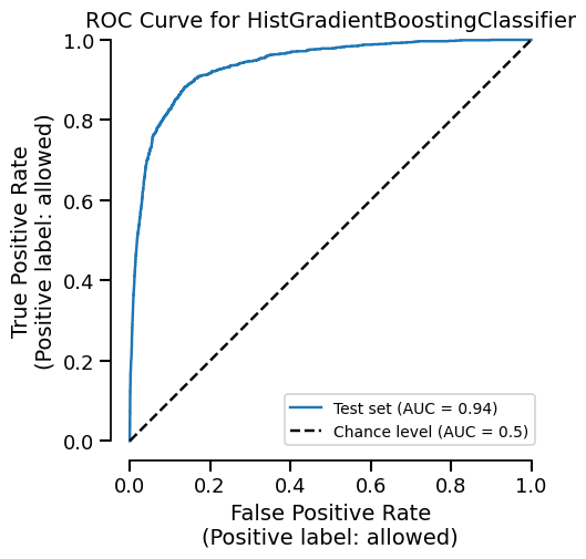
Time taken: 0.01 seconds

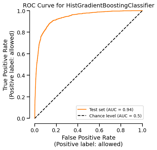
We only use the cache to retrieve the display object and not directly the matplotlib figure. It means that we can still customize the cached plot before displaying it:

display.plot(roc_curve_kwargs={"color": "tab:orange"})

Be aware that we can clear the cache if we want to:

report.clear_cache()
report._cache

{}

It means that nothing is stored anymore in the cache.

Caching with CrossValidationReport

CrossValidationReport uses the same caching system for each split in cross-validation by leveraging the previous EstimatorReport:

from skore import CrossValidationReport

report = CrossValidationReport(model, X=df, y=y, splitter=5, n_jobs=4)
report.help()

╭───────────── Tools to diagnose estimator HistGradientBoostingClassifier ─────────────╮
│ CrossValidationReport                                                                │
│ ├── .metrics                                                                         │
│ │   ├── .accuracy(...)         (↗︎)     - Compute the accuracy score.                 │
│ │   ├── .brier_score(...)      (↘︎)     - Compute the Brier score.                    │
│ │   ├── .log_loss(...)         (↘︎)     - Compute the log loss.                       │
│ │   ├── .precision(...)        (↗︎)     - Compute the precision score.                │
│ │   ├── .precision_recall(...)         - Plot the precision-recall curve.            │
│ │   ├── .recall(...)           (↗︎)     - Compute the recall score.                   │
│ │   ├── .roc(...)                      - Plot the ROC curve.                         │
│ │   ├── .roc_auc(...)          (↗︎)     - Compute the ROC AUC score.                  │
│ │   ├── .timings(...)                  - Get all measured processing times related   │
│ │   │   to the estimator.                                                            │
│ │   ├── .custom_metric(...)            - Compute a custom metric.                    │
│ │   └── .summarize(...)                - Report a set of metrics for our estimator.  │
│ ├── .cache_predictions(...)            - Cache the predictions for sub-estimators    │
│ │   reports.                                                                         │
│ ├── .clear_cache(...)                  - Clear the cache.                            │
│ ├── .get_predictions(...)              - Get estimator's predictions.                │
│ └── Attributes                                                                       │
│     ├── .X                             - The data to fit                             │
│     ├── .y                             - The target variable to try to predict in    │
│     │   the case of supervised learning                                              │
│     ├── .estimator                     - Estimator to make the cross-validation      │
│     │   report from                                                                  │
│     ├── .estimator_                    - The cloned or copied estimator              │
│     ├── .estimator_name_               - The name of the estimator                   │
│     ├── .estimator_reports_            - The estimator reports for each split        │
│     ├── .ml_task                       - No description available                    │
│     ├── .n_jobs                        - Number of jobs to run in parallel           │
│     ├── .pos_label                     - For binary classification, the positive     │
│     │   class                                                                        │
│     ├── .split_indices                 - No description available                    │
│     └── .splitter                      - Determines the cross-validation splitting   │
│         strategy                                                                     │
│                                                                                      │
│                                                                                      │
│ Legend:                                                                              │
│ (↗︎) higher is better (↘︎) lower is better                                             │
╰──────────────────────────────────────────────────────────────────────────────────────╯

Since a CrossValidationReport uses many EstimatorReport, we will observe the same behaviour as we previously exposed. The first call will be slow because it computes the predictions for each split.

start = time.time()
result = report.metrics.summarize().frame()
end = time.time()
result

		HistGradientBoostingClassifier
		mean	std
Metric	Label / Average
Precision	allowed	0.432482	0.123726
	disallowed	0.959970	0.005586
Recall	allowed	0.423435	0.097387
	disallowed	0.951590	0.043077
ROC AUC		0.874609	0.030393
Brier score		0.063774	0.033356
Fit time (s)		16.128872	3.197235
Predict time (s)		2.083737	0.450096

print(f"Time taken: {end - start:.2f} seconds")

Time taken: 11.60 seconds

But the subsequent calls are fast because the predictions are cached.

start = time.time()
result = report.metrics.summarize().frame()
end = time.time()
result

		HistGradientBoostingClassifier
		mean	std
Metric	Label / Average
Precision	allowed	0.432482	0.123726
	disallowed	0.959970	0.005586
Recall	allowed	0.423435	0.097387
	disallowed	0.951590	0.043077
ROC AUC		0.874609	0.030393
Brier score		0.063774	0.033356
Fit time (s)		16.128872	3.197235
Predict time (s)		2.083737	0.450096

print(f"Time taken: {end - start:.2f} seconds")

Time taken: 0.00 seconds

Hence, we observe the same type of behaviour as we previously exposed.